Introduction

Welcome to the fabled third part of Documentation Tips of Game Designers! The first part was all about theory, the second part was 50% theory and 50% practical tips on Google Docs, this time we are going full practice with Google Sheets.

To be clear, it’s impossible for me to write everything about Spreadsheets right here - this is going to be an introduction that will give the readers some tools that should be enough to kickstart the process of learning how to use them.

About the differences between Google Sheets and Microsoft Excel: they’re mostly the same, Google Sheets has less features than Excel, but it has Plugins to make up for it. As always, I’ll be explaining Google Sheets since it’s going to be what most of the readers will be able to use, but everything can still be applied in any Spreadsheet editor.

A small love letter to spreadsheets

Spreadsheets are feared by many, and rightly so I may add. Creating a Spreadsheet is not easy, and you need to write some code to use them properly, but they are well worth the investment.

Remember how I explained that Documents don’t bring forth the development of your game, but they are an investment to be faster during production? Well, Spreadsheets are an amazing investment.

You can use them for tuning of your game’s Progression, Economy and Stats, to analyze your competitors and gather data from there, to make sure that you are on budget or organize your team’s work. They are a giant and automatic table, and you know how good tables are (if you read my second article, *wink wink*).

The basics of Google Sheets

Let’s start with the basics of the basics. Before even starting your Spreadsheet you need to organize your ideas into rows and columns. Let’s make a small dictionary: elements are the single pieces you are analyzing in your document, like competitor games, your game’s enemies or the character stats; data are the specific stats that each element has, so for example: a competitor game (element) might have these data: sell count, positive reviews counts, metacritic, steam tags, cost and more, if needed.

Ideally, you want to organize elements in rows and their data in columns, and you want to keep the columns on a single screen window, since it’s easier to scroll down than it is to move left and right - keep in mind that Google Sheets doesn’t adapt to screen resolution, so different screen will show a different amount of columns.

Some quick tips to help your document look better:

Now, let’s explore some more commonly used and powerful features for your Design Documents:

Conditional Formatting

How it works

Highlight the cells you want to add Conditional Formatting to (typically a whole column), right click and select “Conditional Formatting” at the bottom of the menu.

You can decide what formatting (i.e. fill color, font style) the cells in the range will have based on a criteria you choose. By clicking on “Color scale” you can give cells a gradient based on their value.

Custom formula is a particularly good criteria since it allows you to script the criteria yourself; just be warned that there is no autocompile, so you might want to test the formula in a cell and then copy paste it. Also, syntax is a bit weird, so you might need to troubleshoot.

When to use it

You need to see what’s the biggest element in a list? Use a gradient conditional formatting, this way you’ll be able to quickly find what you need.

You want to check if you have a duplicate anywhere in a column? Use a conditional formatting with “custom formula” using this formula right here: =countif(A:A,A1)>1.

Do you have a Traffic Light document with tasks that can be Done, WiP or Cut? Add conditional formatting that automatically colors the cells containing those words in Green, Yellow and Red - even better if you use Data Validation!

Data validation

How it works

Just like Conditional Formatting, right click on the selected range and click on “Data Validation” at the bottom of the menu. This creates a drop down menu on the cells, containing the data you want to. There are many criteria, but the main ones are:

When to use it

Remember the Traffic Light I talked about with Conditional Formatting? What if Done, WiP and Cut are words chosen from a Data Validation menu? This way, anyone using the document will use the right syntax and the Conditional Formatting will work as intended.

Do you want to have a dynamically changing Data validation that doesn’t require to edit the whole column each time? By selecting “Items from a range” you’ll be able to add the items directly on the document itself, maybe even importing it from different places.

You want to check which and how many games you are analyzing are on Steam? Add a “is on Steam” Column and put a checkbox in there. Pro tip: with the custom formula “=TRUE” in Conditional Formatting, true checkboxes will change color!

Formulas

Formulas are what make Spreadsheets so amazing. They are definitely not quantum physics, but they do require a bit of a mathematical mindset to properly use them.

To create a Formula you’ll have to type “=” inside any cell, at which point the cell is going to automatically expect a Formula. The “=” sign is basically saying to that cell that it should be containing “this data”, in which “this data” can be the result of various mathematical operations, the result of Google Sheets built-in Functions or even just the value of a different cell.

To quickly show what I mean and get everyone accustomed to this: write something in the cell A1; then, write in the cell B1 “=A1” - the same word should appear in both the cells. Now, by changing the text in A1, B1 will change as well. Let’s move it up an inch: write a number in A1, and a number in B1; now, write in C1 the formula “=A1+B1” - the value in C1 is the sum of those two values.

Tip: by dragging a formula, it will auto compile itself in the other cells - what this means is that if you drag down the previously made formula by selecting the cells A1, B1 and C1, the formula will automatically update (and the numbers should increase). By adding a $ sign in front of the letter, number or both in the formulas, you can prevent this from happening (like "=$A$1+$B$1")!
Here’s a quick rundown of some useful Functions in Google Sheets:

Final boss: Arrays

I should mention Arrays, since they can be of great help in creating documents that are easy to use. What they do is essentially collect inside a single cell the information that needs to be written down a range of cells. This is incredibly useful for formulas that might break when adding rows or columns to the spreadsheet - the Array will automatically fill and fix the values inside of them. They are a bit hard, so I won’t be explaining them here, but it is definitely something to study for anyone interested.

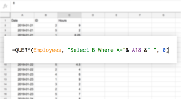
Secret boss: Queries

And I must mention Queries. QUERY is the most powerful function in Google Sheets: it allows you to use a Structured Query Language to script behaviours in your spreadsheets. This is hard programming, so using them is a big investment in both time and work, but it will give any document an edge. To follow the trend of this article, they are mostly useful in… well, anything really.

Charts: their own thing

To briefly touch charts, they are their own thing really. There is a field of study completely dedicated to how to display data, so trying to cover it here would be useless - it is a topic that really fascinates me though, so one day I might make an article solely dedicated to Charts! You can add them by clicking on Insert>Chart. If you select a range of cells first, Google Sheets will make a chart with those, if not it will try to figure it out by itself. 

Conclusions

Well, this was a ride. When I started this series I wasn’t sure it would work out so well, and I didn’t even think someone would find it useful, but I’m glad I was wrong. Like last time, I highly suggest everyone to add me on LinkedIn to ask questions and chat!

Meeting new people was my goal all along, so I look forward to talking with anyone!

Thank you all for your time!