The physics of trains in Assassin's Creed Syndicate

In this article, I would like to present our custom simulator which we created to model the physics of trains in Assassin's Creed Syndicate. The game is set in the year 1868 in London during the times of the industrial revolution when steam and steel marked the progress of the society. It was a great pleasure to work on this unique opportunity of bringing to life the world of Victorian Era London. Attention to the historical and the real-world details led us to the creation of this physically-based simulation.

Introduction

It is not common these days to write your own physics engine. However, there are situations when it is very useful to create your own physical simulator from the ground up. Such situations might occur when there are specific conditions or needs for a new gameplay feature or a part of the simulated game world. This is the situation which we came across when developing railway system and the whole management of trains running in the 19^th-century London.

The standard coupling system for trains in Europe is presented in figure 1 on the left. The same system was used in 19^th-century trains in London [1]. When we started our work on trains we quickly realized that we can create interesting interactions and behaviors when physically simulating the chain. So instead of having rigidly connected wagons, we have them connected with the movable coupling chain which drives the movement for all wagons in the train.

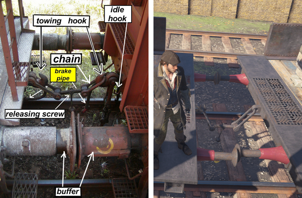
Figure 1. Chain coupler details on the left (source: Wikipedia [1]). The coupling system in Assassin’s Creed Syndicate on the right.

There are a couple of advantages for our own physics solution in this case:

Here is the video with our physics of trains in action:

We will start with the section explaining first how we control our trains.

Note:

To simplify our discussion, we use the word “tractor” to describe a wagon closer to the locomotive and the word “trailer” to describe a wagon closer to the end of the train.

Controlling locomotive

We have a very simple interface to control the locomotive – which consists of requesting a desired speed:

Locomotive::SetDesiredSpeed(float DesiredSpeed, float TimeToReachDesiredSpeed)

Railway system manager submits such requests for every train running in the game. To execute the request, we calculate a force needed to generate desired acceleration. We use the following formula (Newton’s second law):

where F is computed force, m is the locomotive’s mass, , and t = TimeToReachDesiredSpeed.

Once the force is calculated, we send it to WagonPhysicsState as an “engine force” to drive the locomotive (more information about it in the next section).

Because the physical behavior of the train can depend for example on the number of wagons (wagons colliding with each other creating a chain reaction and pushing the train forward), we need a way to ensure that our desired speed request once submitted is fully executed. To achieve this, we re-evaluate the force needed to reach desired speed every 2 seconds. This way we are sure that the request once submitted is finally reached. But as a result, we are not able to always satisfy TimeToReachDesiredSpeed exactly. However, small deviations in time were acceptable in our game.

Also, to keep the speed of the locomotive as given by SetDesiredSpeed request, we do not allow the coupling chain constraint to change the speed of the locomotive. To compensate the lack of such constraint impulses, we created a special method to model the dragging force – more about it in the section “the start-up of the train”. Finally, we do not allow collision response to modify the speed of the locomotive except when the train decelerates to a zero speed.

In the next section, we describe our basic level of the physical simulation.

Basic simulation step

This is a structure used to keep physical information about every wagon (and locomotive):

struct WagonPhysicsState
{
    // Values advanced during integration: 
    // distance along the track and momentum.
    RailwayTrack m_Track;
    float m_LinearMomentum;

    // Speed is calculated from momentum.
    float m_LinearSpeed;

    // Current value of forces.
    float m_EngineForce;
    float m_FrictionForce;

    // World position and rotation obtained directly from the railway track.
    Vector m_WorldPosition;
    Quaternion m_WorldRotation;

    // Constant during the simulation:
    float m_Mass;
}

As we can see there is no angular velocity. Even if we check collisions between wagons using 3D boxes (with rotation always aligned to the railway line) trains are moving in the 1D world along the railway line. So there is no need to keep any information about the angular movement for the physics. Also, because of the 1D nature of our simulation, it is enough to use floats to store physical quantities (forces, momentum and speed).

For every wagon we use Euler method [2] as a basic simulation step (dt is the time for one simulation step):

void WagonPhysicsState::BasicSimulationStep(float dt)
{
    // Calculate derivatives.
    float dPosition = m_LinearSpeed;
    float dLinearMomentum = m_EngineForce + m_FrictionForce;

    // Update momentum.
    m_LinearMomentum += dLinearMomentum*dt;
    m_LinearSpeed = m_LinearMomentum / m_Mass;

    // Update position.
    float DistanceToTravelDuringThisStep = dPosition*dt;
    m_Track.MoveAlongSpline( DistanceToTravelDuringThisStep );

    // Obtain new position and rotation from the railway line.
    m_WorldPosition = m_Track.GetCurrentWorldPosition();
    m_WorldRotation = m_Track.AlignToSpline();
}

We use three main equations to implement our BasicSimulationStep. These equations state that velocity is a derivative of position and force is a derivative of momentum (dot above the symbol indicate derivative with respect to time) [2 - 4]:

The third equation defines momentum P, which is a multiplication of mass and velocity:

In our implementation, applying an impulse to the wagon is just an addition operation to the current momentum:

void WagonPhysicsState::ApplyImpulse(float AmountOfImpulse)
{
    m_LinearMomentum += AmountOfImpulse;
    m_LinearSpeed = m_LinearMomentum / m_Mass;
}

As we can see, immediately after changing momentum we are recalculating our speed for an easier access to this value. This is done in the same way as in [2].

Now, when we have the basic method to advance the time in our simulation, we can move forward to the other parts of our algorithm.

High-level steps of the simulation for one train

Here is the pseudo code for the full simulation step for one train:

// Part A
Update train start-up velocities

// Part B
For all wagons in train
    ApplyDeferredImpulses

// Part C
For all wagons in train
    UpdateCouplingChainConstraint

// Part D
For all wagons in train
    UpdateEngineAndFrictionForces
    SimulationStepWithFindCollision
    CollisionResponse

It is important to mention that, as it is written in the pseudo-code, every part is executed consecutively for all wagons in one train. Part A implements specific behavior related to the start-up of the train. Part B applies deferred impulses that come from collisions. Part C is our coupling chain solver – to be sure that we do not exceed maximum distance for the chain. Part D is responsible for engine and friction forces, the basic simulation step (integration) and handling collisions.

In our simulation algorithm, we always keep the same order of updates for wagons in the train. We start from the locomotive and proceed consecutively along every wagon from the first one to the last one in the train. Because we are able to use this specific property in our simulator, it makes our calculations easier to formulate. We use this characteristic especially for collision contact – to consecutively simulate every wagon’s movement and check collisions only with one other wagon.

Every part of this high-level simulation loop is explained in details in the following sections. However, because of its importance, we start with part D and SimulationStepWithFindCollision.

Simulation with collisions

Here is the code for our function SimulationStepWithFindCollision:

WagonPhysicsState SimulationStepWithFindCollision(WagonPhysicsState InitialState, float dt)
{
    WagonPhysicsState NewState = InitialState;
    NewState.BasicSimulationStep( dt );
    bool IsCollision = IsCollisionWithWagonAheadOrBehind( NewState );
    if (!IsCollision)
    {
        return NewState;
    }
    return FindCollision(InitialState, dt);
}

First, we perform tentative simulation step using the full delta time by calling

NewState.BasicSimulationStep( dt );

and checking if in a new state we have any collisions:

bool IsCollision = IsCollisionWithWagonAheadOrBehind( NewState );

If this method returns false, we can use this newly computed state directly. But if we have a collision, we execute FindCollision to find a more precise time and physics state just before the collision event. To perform this task we are using binary search in a similar manner as in [2].

This is our loop to find the more precise time of collision and physics state:

WagonPhysicsState FindCollision(WagonPhysicsState CurrentPhysicsState, float TimeToSimulate)
{
    WagonPhysicsState Result = CurrentPhysicsState;

    float MinTime = 0.0f;
    float MaxTime = TimeToSimulate;
    for (int step = 0 ; step<MAX_STEPS ; ++step)
    {
        float TestedTime = (MinTime + MaxTime) * 0.5f;

        WagonPhysicsState TestedPhysicsState = CurrentPhysicsState;
        TestedPhysicsState.BasicSimulationStep(TestedTime);
        if (IsCollisionWithWagonAheadOrBehind(TestedPhysicsState))
        {
            MaxTime = TestedTime;
        }
        else
        {
            MinTime = TestedTime;
            Result = TestedPhysicsState;
        }
    }

    return Result;
}

Every iteration gets us closer to the precise time of the collision. We also know that we need to check our collisions only with one wagon directly ahead of us (or behind us in a case of backward movement). Method IsCollisionWithWagonAheadOrBehind uses collision test between two oriented bounding boxes (OBB) to provide the result. We are checking collisions in a full 3D space using m_WorldPosition and m_WorldRotation from WagonPhysicsState.

Collision response

Once we have found the state of physics just before the collision event, we need to calculate appropriate reaction impulse j to apply it to both tractor and trailer wagons. First, we start with a calculation for current relative velocity between wagons before the collision:

A similar value of relative velocity  but after the collision event:

where  and  are velocities after the collision response impulse j is applied. These velocities can be calculated using velocities from before the collision and our impulse j as follows ( and  are wagon’s masses):

We are ready now to define the coefficient of restitution r:

The coefficient of restitution describes how “bouncy” the collision response is. Value r = 0 means a total loss of energy, value r = 1 means no loss of energy (perfect bounce). Substituting into this equation our previous formulas we get

Organizing this equation to get our impulse j:

Finally, we can calculate our impulse j:

In our game, we use r = 0.35 as the coefficient of restitution.

We apply impulse +j to the tractor and impulse -j to the trailer. However, we use “deferred” impulses for the tractor. Because we already processed integration for our tractor and we do not want to change its current velocity, we defer our impulse to the next simulation frame. It does not create any significant change in visual behavior as one frame difference is very hard to notice. This “deferred” impulse is collected for the wagon and applied during part B in the next simulation frame.

A video showcasing the stop of the train:

Coupling chain

We can think about the coupling chain as a distance constraint between wagons. To keep this distance constraint satisfied we compute and apply appropriate impulses to change velocities.

We start our calculations with a distance evaluation for the next simulation step. For every two wagons connected by a coupling chain, we calculate distances they will travel during the upcoming simulation step. We can compute such distance very easily using current velocity (and inspecting our integration equations):

where x is our distance to travel, V is current velocity and t is the simulation step time.

Then, we calculate the formula:

where:

 = distance the tractor will travel during upcoming simulation step.

 = distance the trailer will travel during upcoming simulation step.

If FutureChainLength is bigger than the maximum length of the coupling chain, then our distance constraint will be broken after the next simulation step. Let assume that

If distance constraint is broken, d value will be positive. In such case, to satisfy our distance constraint we need to apply such impulses that d = 0. We will use the wagon’s mass to scale appropriate impulses. We want the lighter wagon to move farther and the heavier wagon to move less. Let us define coefficients  and  as follows

Please notice that . We want the trailer to move with the additional distance  and the tractor with the distance  during the next simulation step. To accomplish it by applying an impulse we need to multiply the given distance by mass divided by the simulation step time:

If we will use additional symbol C defined as follows

we can simplify these impulses to

We can see that they have equal magnitude but the opposite sign.

After applying both impulses, wagons connected with this coupling chain will not break the distance constraint during the next simulation step. These impulses modify velocities in such way that integration formulas will end up at positions satisfying the maximum distance for the chain.

Still, after computing these impulses for one coupling chain, we can possibly break the maximum chain distance for other wagons in a train. We would need to rerun this method several times to converge to the final solution. However, in practice, we run this loop just once. It is enough to achieve good global results.

We execute these calculations consecutively for every coupling chain in a train starting from the locomotive. We always apply impulses to both wagons connected with the chain. But there is one exception to this rule: we never apply an impulse to the locomotive. We want the locomotive to keep its speed, so we apply impulse only to the first wagon after the locomotive. This impulse applied only to the trailer needs to compensate for the whole required distance d (in such case we have ,  and ).

Correction during sharp curves

Because our simulation runs along the 1D line we have problems with a perfect fit for the coupling chain on the hook when wagons are running on a sharp curve. This is the situation when our 1D world meets 3D game world. Our coupling chain is finally placed in the 3D world, but our impulses (to compensate for the distance constraint) are applied only in our simplified 1D world. To correct the final placement of the chain on the hook we slightly modify MaximumLengthOfCouplingChain depending on the relative angle between directions of the tractor and the chain. Bigger the angle, smaller the maximum available length of the chain. First, we compute dot product between two normalized vectors:

where  is the normalized direction of the coupling chain and  is the forward direction of the tractor. Then, we use the following formula to finally compute the distance we want to subtract from the physical length of the coupling chain:

float DistanceConvertedFromCosAngle = 2.0f*clamp( (1.0f-s)-0.001f, 0.0f, 1.0f );
float DistanceSubtract = clamp( DistanceConvertedFromCosAngle, 0.0f, 0.9f );

As you can see we do not calculate the exact value of the angle, as we use cosine angle directly. It saves us some processing time and is sufficient for our needs. We also use some additional numbers, based on empirical tests – to limit values within reasonable thresholds. Finally, we use DistanceSubtract value before starting to satisfy the distance constraint for the coupling chain:

MaximumLengthOfCouplingChain = ChainPhysicalLength - DistanceSubtract;

It turns out that these formulas work very well in practice. It makes our coupling chain hanging correctly on the hook even on sharp turnings along the railway curves.

Now, we will describe specific case of the start-up of the train.

The start-up of the train

As mentioned before, we are not allowing the coupling chain impulses to change the speed of the locomotive. However, we still need a way to simulate effects of a dragging force - especially during the start-up of the train. When locomotive starts it drags other wagons, but also the locomotive itself should slow down according to the dragging mass of wagons. To achieve this, we modify velocities when the train accelerates from a zero speed. We start with calculations based on the law of conservation of momentum. This law states that “the momentum of a system is constant unless external forces act on that system” [3]. It means that in our case the momentum  before dragging another wagon, should be equal to the momentum  just after the coupling chain is pulling another wagon:

In our case, we can expand it to the following formula:

where  is the mass of the i-th wagon ( is the mass of the locomotive),  is the current speed of the locomotive (we assume that all already moving wagons have the same speed as the locomotive),  is the speed of the system after the dragging (we assume that all dragged wagons will have the same speed). If we use additional symbol  defined as follows

we can simplify our formula in this way

 is the value we are looking for:

Using this formula, we simply set the new velocity  for the locomotive and for all wagons (from 2 to n) currently being dragged by the coupling chain.
In figure 2 below we can see the schematic description when the locomotive  and two wagons start to drag the third wagon :

Figure 2. The start-up of the train.

Here is the video with the start-up of the train:

Friction

To compute friction force (variable m_FrictionForce in WagonPhysicsState) we are using formulas and values chosen after a series of experiments to better support our gameplay. We have constant friction force value, but additionally, we are scaling it according to the current speed (when the speed is below 4). Here is the graph of our standard friction force for wagons:

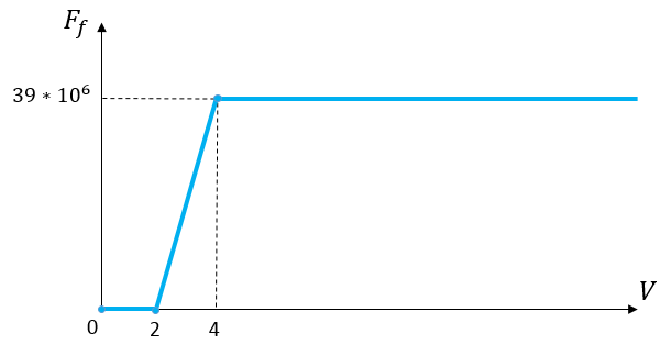
Figure 3. The standard friction force for wagons.

We use different friction values for detached wagons:

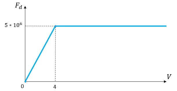
Figure 4. The friction force for detached wagons.

Additionally, we want to allow the player to easily jump between wagons during a short amount of time after the detaching. So, we use a smaller value of the friction and we scale it with the time passing from the detaching event. The final value of the friction for detached wagons is given by:

where t is time passed from the detaching event (measured in seconds).

As we can see, we use no friction during the first 3 seconds and then gradually increase it.

Final remarks

In our trains, we also have movable bumpers at the front and the back of every wagon. These bumpers do not generate any physical forces. We implemented their behavior as an additional visual element. They move according to the detected displacement of a neighbor bumper in another wagon.

Also, as you can notice, we are not checking collisions between different trains in our simulator. It is the responsibility of the railway system manager to adjust trains speed to prevent collisions. In our simulation, we check collisions between wagons only within one train.

It is important to mention that for the high-quality perception of trains in the game sounds and special effects play a very important role. We are calculating different quantities derived from the physical behaviors to control sounds and FXs (like sounds for the tension of the coupling chain, bumpers hit, deceleration, etc.). 

Summary

We presented our custom physically-based simulator for trains created for Assassin’s Creed Syndicate. It was a great pleasure and a big challenge to work on this part of the game. In the open-world experience, there are a lot of gameplay opportunities and different interactions. It creates even more challenges to deliver stable and robust systems. But in the end, it is very rewarding to observe trains running in the game and contributing to the final quality of the player’s experience.

Thanks

I would like to thank James Carnahan from Ubisoft Quebec City and Nobuyuki Miura from Ubisoft Singapore for reviewing this article and useful advice.

I would like to thank my colleagues at Ubisoft Quebec City studio: Pierre Fortin - who let me start with the physics of trains and inspired to push it forward; Dave Tremblay for his technical advice; James Carnahan for every talk about physics we did together; Matthieu Pierrot for his inspiring attitude; Maxime Begin who was always happy to start a talk about programming with me; Vincent Martineau for every help I have received from him. I would like also to thank Martin Bedard, Marc Parenteau, Jonathan Gendron, Carl Dumont, Patrick Charland, Emil Uddestrand, Damien Bastian, Eric Martel, Steve Blezy, Patrick Legare, Guillaume Lupien, Eric Girard and every other person who worked on Assassin’s Creed Syndicate for making such incredible game!

References

[1] “Buffers and chain coupler”, https://en.wikipedia.org/wiki/Buffers_and_chain_coupler

[2] Andrew Witkin, David Baraff and Michael Kass, “An Introduction to Physically Based Modeling”, http://www.cs.cmu.edu/~baraff/pbm/

[3] Fletcher Dunn, Ian Parberry, “3D Math Primer for Graphics and Game Development, Second Edition”, CRC Press, Taylor & Francis Group, 2011.

[4] David H. Eberly, “Game Physics. Second Edition”, Morgan Kaufmann, Elsevier, 2010.