I recently had the opportunity to speak at Spark Summit 2019 about one of the exciting machine learning projects that we’ve developed at Zynga. The title of my session was “Automating Predictive Modeling at Zynga with PySpark and Pandas UDFs” and I was able to highlight our first portfolio-scale machine learning project. The slides from my presentation are available on Google Drive.

While we’ve been known for our analytics prowess for over a decade, we’re now embracing machine learning in new ways. We’re building data products that scale to billions of events, tens of millions of users, hundreds of predictive signals, and dozens of games (portfolio-scale). We are leveraging recent developments in Python and Spark to achieve this functionality, and my session provided some details about our machine learning (ML) pipeline. 

The key takeaways from my session are that recent features in PySpark enable new orders of magnitude of processing power for existing Python libraries, and that we are leveraging these capabilities to build massive-scale data products at Zynga. The goal of this post is to provide an overview of my session and details about our new machine learning capabilities. 

I’m a distinguished data scientist at Zynga and a member of the analytics team, which spans our central technology and central data organizations. Our analytics team is comprised of the following groups:

This team picture is from our annual team gathering, called Dog Days of Data.

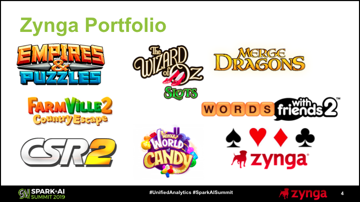
Our portfolio of games includes in-house titles and games from recently acquired studios including Gram Games and Small Giant Games. Our studios are located across the globe, and most teams have embedded analysts or data scientists to support the live operations of our games. One of the goals for the central analytics team is to build data products that any of the games in our portfolio can integrate.

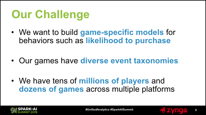
The scale and diversity of our portfolio presents several challenges when building large-scale data products. One of the common types of predictive models built by our data scientists are propensity models that predict which users are most likely to perform an action, such as making a purchase.

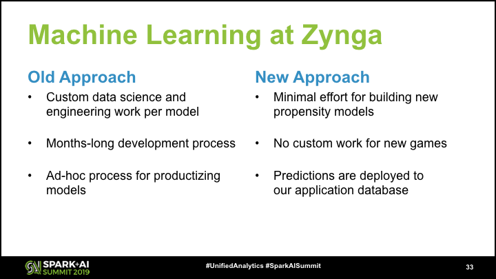
Our old approach for machine learning at Zynga was to build new models for each game and action to predict, and each model required manual feature engineering work. Our games have diverse event taxonomies, since a slots game has different actions to track versus a match-3 game or a card game. 

An additional challenge we have is that some of our games have tens of millions of active users, generating billions of records of event data every day. This means that our predictive models need to scale beyond the single machine setups that we historically used when training models. 

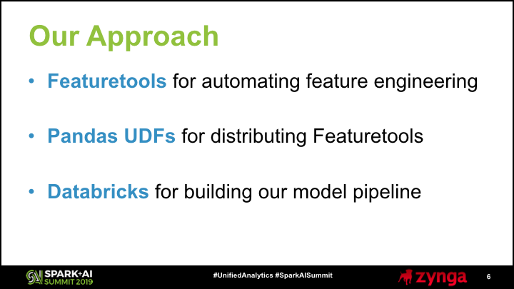
We’ve been able to use PySpark and new features on this platform in order to overcome all of these challenges. The main feature that I focused on for my Spark Summit session is Pandas UDFs (User-Defined Functions), which enable data scientists to use Pandas dataframes in a distributed manner. Another recent tool we’ve been leveraging is the Featuretools library, which we use to perform automated feature engineering. We use Databricks as our Spark environment, and have been able to combine all of these features into a scalable data pipeline that builds hundreds of propensity models daily.

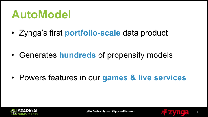
We named the resulting data product AutoModel, because it has enabled us to automate most of the work involved in building propensity models for our games. This is the first portfolio-scale machine learning system at Zynga, which provides predictive models for every one of our games. Given the size of our portfolio and number of responses that we predict, the system generates hundreds of propensity models every day. We use the outputs of AutoModel to personalize our games and live services.

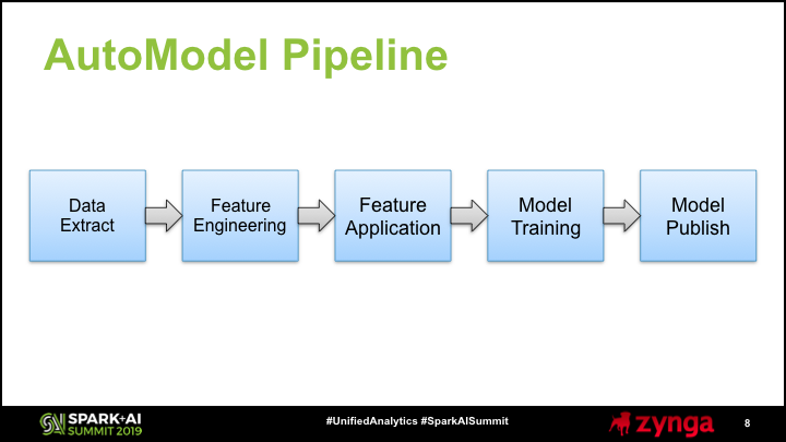
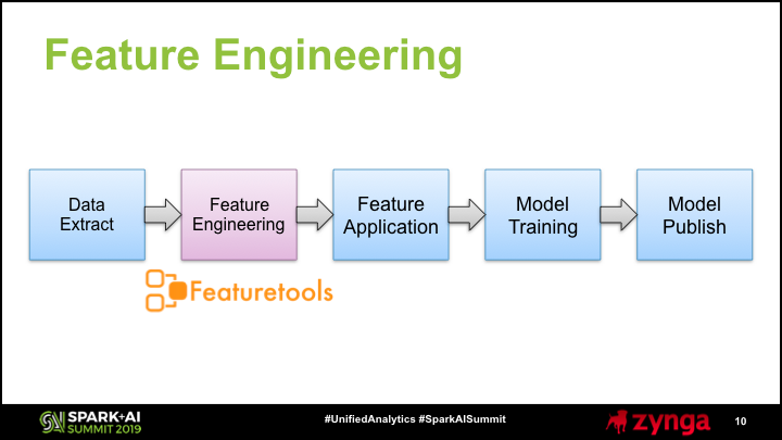
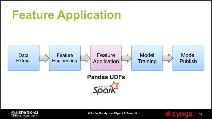
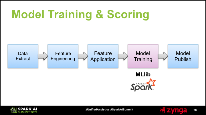
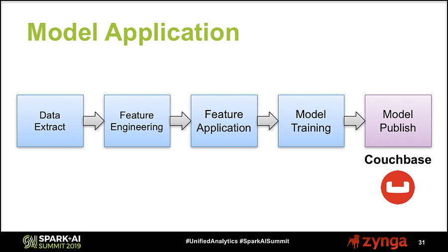
We used PySpark to build AutoModel as an end-to-end data product, where the input is tracking events in our data lake and the output is player records in our real-time database. This slide shows the main components of our Spark pipeline for AutoModel:

We’ll step through each of these components in more detail, and focus on the feature application step, where we apply Pandas UDFs.

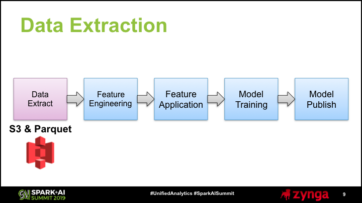
The first phase in our modeling pipeline is extracting data from our data lake and making it accessible as a Spark dataframe. In the initial step, we use Spark SQL to aggregate our raw tracking events into summarized events. The goal of this first step is to reduce tens of thousands of records per player to hundreds of records per player, to make the feature application step less computationally expensive. In the second step, we read in the resulting records from S3 directly in parquet format. To improve caching, we enabled the spark.databricks.io.cache.enabled flag.

The second phase in the pipeline is performing automated feature engineering on a sample of players. We use the Featuretools library to perform feature generation, and the output is a set of feature descriptors that we use to translate our raw tracking data into per-player summaries.

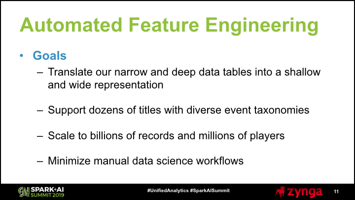
Our primary goal with feature engineering is to translate the different events that occur within a game into a single record per player that summaries their gameplay activity. In our case, we are using structured data (tables) rather than unstructured data such as images or audio. The input is a table that is deep and narrow, which may contain hundreds of records per player and only a few columns, and the output is a shallow and wide table, containing a record per user with hundreds or thousands of columns. The resulting table can be used as input to train propensity models. 

We decided to use automated rather than manual feature engineering, because we needed to build propensity models for dozens of games with diverse event taxonomies. For example, a match-3 game may record level attempts and resulting scores, while a casual card game may record hands played and their outcomes. We need to have a generalizable way of translating our raw event data into a feature vector that summarizes a player.  

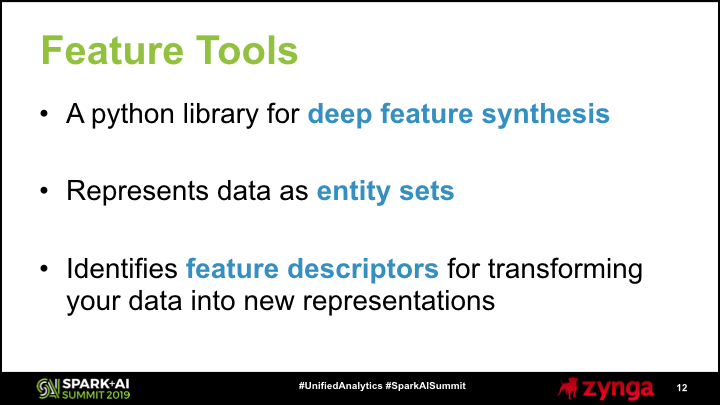
Use used the Featuretools library to automate feature engineering for our data sets. It is a python library that uses deep feature synthesis to perform feature generation. It is inspired by the feature generation capabilities in deep learning methods, but is focused on only feature generation and not model fitting. It generates a wide space of feature transformations and aggregations that a data scientist would explore when manually engineering features, but does so in a programmatic method. 

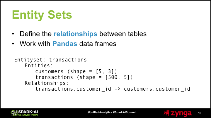
One of the core concepts that the Featuretools library uses is entity sets, which identify the entities and relationships in a data set. You can think of entities as tables, and relationships as foreign keys in a database. The example below shows an entity set for customer and transaction tables, where each customer has zero or more transactions. Describing your data as an entity set enables Featuretools to explore transformations to your data across different depths, such as counting the number of transactions per customer or first purchase date of a customer. 

One of the issues we faced when using this library is that entity sets are backed by Pandas dataframes, and therefore cannot natively be distributed when using PySpark.

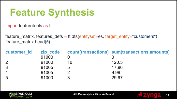
Once you have represented your data as entity sets, you can perform deep feature synthesis to transform the input data sets into an output data set with a single record per target entity, which is a customer for our example. The code below shows how to load the Featuretoools library, perform deep features synthesis (dfs), and output a sample of the results. 

The input to the feature synthesis function is an entity set and a target entity, which is used to determine how to aggregate features. This is typically the root node in your entity set, based on your foreign key constraints. The output of this code shows that a single record is created for each customer ID, and the columns include attributes from the customer table (zip code) and aggregated features from the related tables, defined here as the number and total value of transactions. If additional relationships are added to the entity set, even more features can be generated at different depths. In this case, the customer attributes are at depth 1 and the transaction attributes are at depth 2.

We use Featuretools in AutoModel to perform deep feature synthesis. One of the constraints that we had was that all of the inputs tables in our entity set need to be stored as a single table, and I’ll describe why we had this constraint later on. Luckily, our data is already in this format: each event has a player, category, and subcategory field, in additional to other columns that provide additional information. We defined relationships between these columns and split up the input data into multiple tables to define our entities. This allowed us to translate our input table representation into an entity set representation with a depth of 3. 

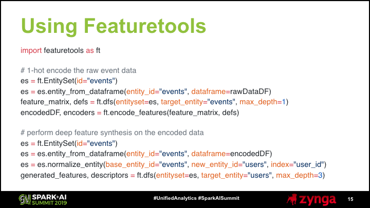
For the feature generation phase, we use sampled data sets to ensure that Featuretools can run on a single machine, which is the driver node in our PySpark workflow. We also use a two-step encoding process that first performs 1-hot encoding on our input table and then performs deep feature synthesis on the encoded table. 

The code snippet below shows some of the details involved in performing this transformation. We create an events entity set using our raw input data, using feature synthesis with a depth of 1 to create a set of feature descriptors (defs), and then use encode_features to perform 1-hot encoding. In the second step, we use the resulting dataframe (encodedDF) as input to deep feature synthesis with a depth of 3. The result of this code block is a transformed dataframe with our generated features, and a set of feature descriptors that we can use to transform additional dataframes. One of the steps omitted in this block is the definition of the relationships in our entity set.

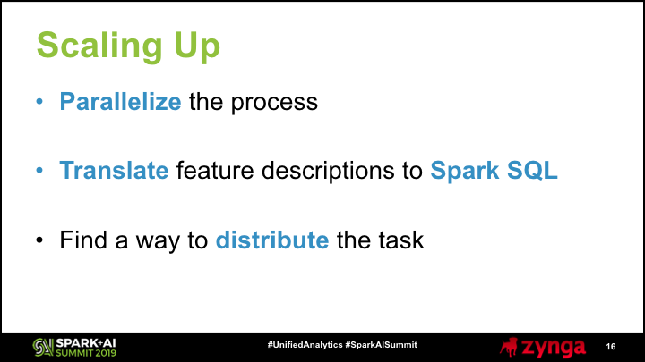
When we first tried out Featuretools on a sample of our data, we were excited to see how well the models performed that we trained using the generated features. But we had a problem, we needed to scale up from tens of thousands to tens of millions of users in order for this approach to work in production. 

We needed a way to both parallelize and distribute the feature application process across a cluster of machines. Our initial approach was to translate the feature descriptor objects output by Featuretools into Spark SQL code that we could run against our raw input data. However, we found that using this approach was too slow when generating thousands of different features. It also meant that we could not support all of the feature transformations available, such as skew. Our solution to this problem is to use Pandas UDFs to support all of the feature transformations provided by Featuretools, while also distributing the task across a Spark cluster.

The third phase in our pipeline is applying the feature generation step to tens of millions of users, and is the focus of this post. We were able to take an existing Python library that works only with Pandas dataframes and scale it to hundreds of machines in a PySpark cluster. To accomplish this task, we used a new feature in Spark that enables distributed calculations on Pandas dataframes, and were able to scale to our full data set.

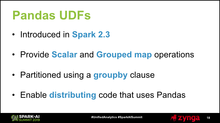
The enabling feature in PySpark that allowed us to realize this new scale in computation is Pandas UDFs. We are using the grouped map feature, which was introduced in Spark 2.3. In summary, this feature allows you to partition a Spark dataframe into smaller chunks that are converted to Pandas dataframes before being passed to user code. User-defined functions (UDFs) are executed on worker nodes, enabling existing Python code to now be executed at tremendous scale. 

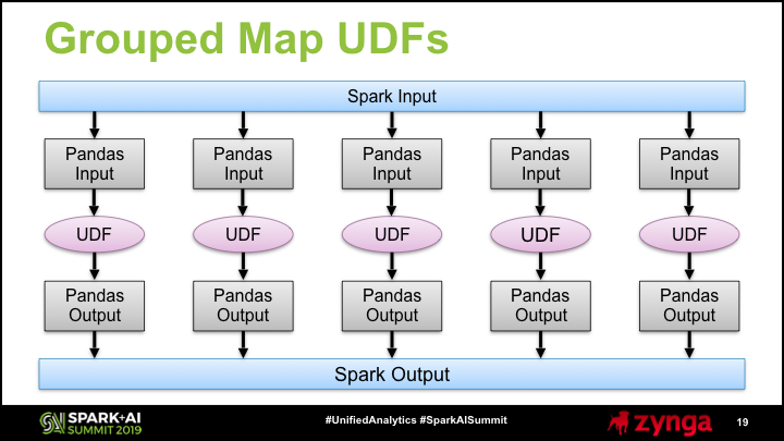
To data scientists writing code with Pandas UDFs, the intent is for the transformation between Spark and Pandas dataframes to be seamless. The input and output of a Pandas UDF is a Spark dataframe. To use a UDF, you specify a partition value in a groupby statement, and pass a function that takes a Pandas dataframe as input and outputs a new Pandas dataframe. This feature enables data scientists to define how to partition a problem, use well-known Python libraries to implement the logic, and achieve massive scale. The figure below visualizes how Pandas UDFs enable large Spark dataframes to be decomposed into smaller objects, transformed with user code, and then recombined into a new Spark frame.

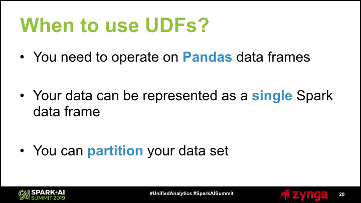
Pandas UDFs are a powerful feature in PySpark, enabling distributed execution of Python code. However, a few conditions need to be met for a problem to match this use case. The first prerequisite is that your data can be well partitioned by a key, and the second prerequisite is that your data needs to be represented as a single Spark dataframe. The grouped map feature is able to distribute a single dataframe across worker nodes using a partitioning key, and only supports the groupby operation on a single object. I mentioned this constraint in slide 15, and our data representation fits this condition. 

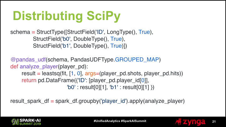
The introduction post on Pandas UDFs shows how to use the ordinary least squares (OLS) function in the statsmodel package in a distributed mode. We’ll use a similar function for this post, the leastsq function in SciPy. Neither of these functions were coded to natively operate in a distributed mode, but Pandas UDFs enable these types of functions to scale as long as you can subdivide your task with a partition key. 

The example below works with the Kaggle NHL (Hockey) data set, which describes a number of different games for each active player on an NHL roster since 2007. The goal of this UDF is to determine if there is a relationship between goals and hits in the NHL, based on a simple linear model fit. 

There are four key steps to using a Pandas UDF:

The result of this code snippet is that the NHL data set can be distributed across a Spark cluster to perform the leastsq function on a large set of players. 

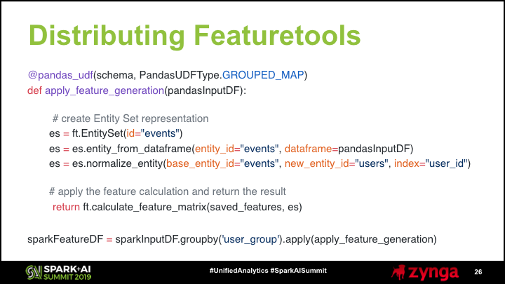
We use Pandas UDFs in combination with the Featuretools library to perform feature generation on tens of millions of users. The code snippet below shows how we partition our active player base into dataframes that can fit into memory on our worker nodes in order to perform deep feature synthesis. 

One of the challenges with using a Pandas UDF is that you can only pass a single object as input. However, you are able to use global variables that have been instantiated on the driver node, which are the feature transformations (saved_features) that we generated during our feature engineering phase of our pipeline. We also generated a schema object during this step by sampling a single row from the transformed data set, converting the result to a Spark dataframe, and retrieving a schema object using df.schema.

This code snippet omits a few details that are necessary for setting up entity sets and performing two-phase feature synthesis, where we perform 1-hot encoding and then run deep feature synthesis. However, the takeaway is to show how you can use libraries such as Featuretools, which require Pandas dataframes, and scale them to massive data sets.

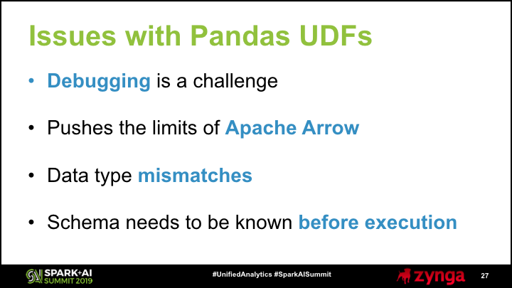
Pandas UDFs can be extremely valuable when building machine learning pipelines, but there are also risks involved in using this feature. The first issue that we encountered was that debugging Pandas UDFs was much more difficult than working with Pandas dataframes on the driver node, because you can no longer use print statements to trace execution flow within a notebook environment, and instead have to browse through log files to trace the output of your code. Our approach for testing Pandas UDFs is to first use toPandas() on a small dataframe and write a groupby apply function that runs on the driver node before trying to distribute the operation. 

The second type of issues that we faced were more difficult to debug, because they occurred only when using UDFs and not when testing locally on the driver node. These problems resulted from issues with Apache Arrow and data type mismatches, since Spark uses Arrow as an intermediate representation between Spark and Pandas dataframes. We ran into an issue with Apache Arrow, which was resolved by upgrading our version of PyArrow. However, we also ran into issues with data type mismatches, such as float16 not being supported. Our workaround for this issue was to cast all float data types to a type supported by Arrow. 

One additional challenge we faced was that the schema for the returned Pandas dataframe needs to be specified before the function is defined, since the schema is specified as part of the grouped map annotation. This wasn’t a problem for us, since we separated feature engineering and feature application into separate pipeline phases, but it does mean that the schema of the Pandas UDF needs to be constant and predefined.

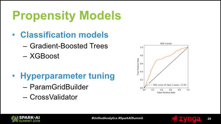
In the fourth phase of our data pipeline, we use the thousands of features that we generated for each game as input to propensity models. For this step, we leverage MLlib to perform feature scaling, hyperparameter tuning, and cross-validation. The output of this step is models that we use to predict player behavior in our games. 

We sample data from prior weeks in order to create a training data set and apply the feature transformations on these players in order to establish baseline metrics for model performance. Our pipeline explores a number of candidate models and selects the best performing model as the champion for making predictions. While XGBoost is not native to MLlib, we’ve integrated it into our pipeline in addition to gradient boosted trees, random forests, and logistic regression. 

The fifth phase in our data pipeline is publishing our propensity model scores to our real-time database. We’ve transformed raw events from our active player base into thousands of features, trained predictive models based on these encodings, and during the last step we finally publish the results.

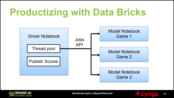
We’ve parallelized AutoModel by running each game as a separate Databricks job. We initially ran the pipeline as a single cluster using the threadpool functionality in the multiprocessing library, but found that spinning up isolated clusters resulted in better stability. Our driver notebook is responsible for spinning up a cluster for each of our games and then publishes the results to our real-time database. We leverage the jobs API in Databricks to execute this process as an automated workflow. 

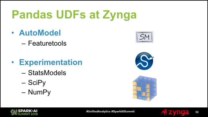
AutoModel is one of several machine learning projects at Zynga where we are utilizing Pandas UDFs to scale Python libraries to large data sets. We are leveraging UDFs to scale our experimentation capabilities, using functions from the SciPy, NumPy, and StatsModels packages. Using Pandas UDFs has enabled us to build notebooks for portfolio-scale experimentation. 

Machine learning has been transformational over the past decade, and Zynga has been exploring recent tools to automate much of our data science workflows. We’ve transitioned from an environment in which data scientists are spending weeks performing manual feature engineering to advanced tools that can automate much of this process. One of the main outcomes of this system is that data scientists are now spending more time with product managers discussing how to improve our games, rather than their models. 

At Zynga, we’ve used Pandas UDF to scale Python libraries to new magnitudes of data sets and have automated much of our propensity modeling pipeline. We’ve built our first portfolio-scale data product and are looking to continue to improve our machine learning expertise. 

Zynga has been adopting Spark as a tool to scale up our data and modeling pipelines. Last year we presented at Spark Summit on predicting retention for new installs and this year we showcased our automated modeling capabilities. If you’re interested in machine learning at Zynga, we are hiring for data science and engineering roles.