Introduction to Caching Shading Information in World Space using Implicit Progressive Low Discrepancy Point Sets

The research presented in this article was done by Matthieu Delaere, Graphics Researcher and Lecturer at DAE Research (HOWEST University of Applied Sciences). The results were used to obtain a master’s degree at the Breda University of Applied Sciences under the supervisor of Dr. ing. Jacco Bikker. This article is a short version of the performed research and serves as an introduction to the topic. It contains some sample code, next to a brief description of the algorithm, which hopefully might help developers and researchers to recreate the prototype in their framework/engine. The publication/thesis can be found on ResearchGate, while the full sample code can be acquired through the following link.

Context

Creating photorealistic computer-generated images involves simulating global illumination which consists of both direct and indirect illumination. Direct illumination replicates the interaction of light with surfaces that are directly visible from a given light source. When light interacts with a surface, it can bounce off and illuminate other surfaces indirectly. The latter effect is called indirect illumination. Both terms are important when trying to create a realistic image. While the direct illumination term in light transport simulation has been successfully translated to real-time applications with a lot of dynamic elements, such as video games, implementing the indirect illumination term while maintaining interactive frame rates remains challenging.

The simulation of global illumination is often based on the rendering equation introduced by Kajiya [1]. While this integral equation describes light transport in a general form, the equation itself is unsolvable because it is infinitely recursive. Even though the equation cannot be solved analytically, the light transport simulation can be approximated using Monte Carlo integration techniques. Monte Carlo integration can produce realistic images, but it is often computational expensive. The image quality also depends on the number of samples taken and the distribution of those samples. While numerous studies improved the convergence rates of Monte Carlo methods, by using techniques such as importance sampling and next event estimation, multiple samples are still required to achieve a good estimation. To maintain interactive frame rates in real-time applications, it is impossible to take multiple samples per pixel (SPP) within a frame to estimate the indirect illumination of a point using current generation hardware.

One way to solve this problem is by spreading the calculations over multiple frames. This requires the intermediate results, which represents shading information, to be cached in a data structure. Most current techniques store the information in a 2D texture, effectively storing the information that is currently visible on screen. While these techniques have been proven to be very useful, most suffer from several drawbacks. First, they do not contain information that is offscreen, which can impact the quality of the final image severely. Because the information is stored in a 2D buffer, based on what is currently visible, the data storage is not persistent. This means, whenever we move the camera, parts of our previous calculations are lost as they go out of scope. While this might not be problematic in linear walkthroughs, it is still a shame to lose the results of previous computation time. Finally, whenever a scene contains dynamic elements, reprojection using motion data is required to figure out which pixel from a previous frame relates to a pixel in the current frame.

In offline rendering, this problem is often tackled in a different way. Instead of storing shading information in screen buffers, the information gets stored in 3D points which resides in the virtual scene [2]. In other words, the information gets stored in the closest 3D point, which is part of a 3D point cloud, in world space. This resolves some of the previously mentioned issues. There is no need to use motion data and the data can be stored in a persistent data structure. Although this technique is powerful, it often requires a pre-processing step to create the 3D point set and this point set takes up a lot of memory.

In the last few years, researchers have been investigating how to translate this technique to real-time applications, while keeping the memory footprint as low as possible. EA SEED [3] introduced a method which takes advantage of their hybrid rendering pipeline to create the point cloud at runtime by spawning surfels (surface elements) using a screen space hole filling algorithm. Even though this technique is extremely powerful, it still requires additional information, which relates to the surfel itself, to be stored (e.g. position, radius, surface normal, etc.).

Our research tries to avoid the storage of this additional information by relying on a hashing scheme, introduced by Nvidia with their path space filtering technique [4], [5]. While Nvidia’s technique is basically performing implicit voxelization using fixed discretization, we use the output of the voxelization to seed a random noise function to generate random 3D points. We are thus trying to combine the power of random point sets with the hashing technique, presented by Nvidia, to lower the memory footprint and to avoid expensive memory lookups by relying on implicitness. Compared to Nvidia’s technique, our technique does not rely on fixed discretization thus lowering potential discretization artifacts. Finally, we reconstruct our final image by filtering the cached data from our data structure, which is also a hash table, in world space instead of relying on screen space reconstruction filters.

In the next section, we will give a brief overview of the algorithm, accompanied with some shader code. The full prototype, which was developed using Microsoft’s MiniEngine framework, is available on Github.

Algorithm

The algorithm consists out of four phases. During the “Implicit Point Generation Pass” the closest random implicit 3D random point is being determined for a given pixel. The data that represents the point (e.g. unique ID) is stored in a temporary 2D buffer. While we determine the closest point, shading information can be calculated in parallel. In the prototype, we use hardware accelerated ray tracing to calculate ambient occlusion (AO), which has similar properties as indirect lighting. Once the closest point for every pixel is found, we accumulate all the shading information in a temporary hash table during an “Accumulation Pass”. This is necessary as multiple pixels can contribute their shading information to the same implicit 3D point. For the accumulation we rely on atomic operations (atomic addition) to guarantee that all the information is correctly added. After this pass, we end up with a small hash table where each entry is unique. This hash table is than merged with the persistent hash table during the “World Caching Pass”. Because every entry is unique, no atomic operations are required. Finally, once the persistent data structure is up to date, we can reconstruct our final image in the “Visualization Pass” by filtering our data in world space using a modified Shepard interpolation [6].

While the passes are mainly there to guarantee the correct synchronization between the data on the GPU, the core of the algorithm is rather simple. An 3D location from our scene, which is reconstructed from our depth buffer, gets discretized and hashed, effectively going from an 3D representation to a unique 1D representation. This unique ID then gets used as a seed value for a random 3D noise generator, again creating a 3D location or point. This point is then also hashed to create a unique 1D index, which is used to find an entry in the persistent hash table. We skip this last step as we use the seed value to find a unique entry in the hash table instead. One can easily add this extra hashing step to make sure it matches the hash table implementation used in their framework. It can also be useful to introduce the extra hashing to achieve better hash table occupancy, which heavily impacts the overall performance.

Implicit Point Generation

The first responsibility of this pass is to discretize the 3D location which we are currently interested in. As mentioned previously, one can acquire the 3D location of a pixel by reconstructing it from the depth buffer. Matt Pettineo has a very nice article about this if you are unfamiliar with the technique. Once we have discretized the location, we use it to create a unique (1D) identifier. We tackle this by representing each axis as a fixed-point value, storing the signed bit in the most significant bit. We then feed these three unsigned integer values in a hash generation function. Based on the research done by Jarzynski et al. [7], we decided to use PCG for this step.

uint GetSeedWithSignedBits(in float3 discretePos, in uint fixedPointFractionalBits)
{
    //Convert float value to fixed point representation for hash functions
    //Putting the signs of all 3 axis in the 3 most significant bits
    const uint fracScale = 1 << fixedPointFractionalBits;
    
    const float3 rawFractionalPart = frac(discretePos);
    const float3 rawIntegerPart = trunc(discretePos);
    
    const uint3 fp = uint3(rawFractionalPart * fracScale); //fractional part
    const uint3 ip = (uint3(abs(rawIntegerPart)) << fixedPointFractionalBits) & 0x1FFFFFFF;
    const uint xp = clamp(sign(rawIntegerPart.x) * -1, 0, 1) << 31;
    const uint yp = clamp(sign(rawIntegerPart.y) * -1, 0, 1) << 30;
    const uint zp = clamp(sign(rawIntegerPart.z) * -1, 0, 1) << 29;
    
    const uint3 fic = fp | ip;
    const uint3 inp = uint3(xp | fic.x, yp | fic.y, zp | fic.z);
    return pcg_nested(inp);
}

Once we have our unique identifier, we use it as a seed value to generate our 3D points. Because we are working with a 3D volume, we use one seed value to generate eight implicit points, one in each subvoxel. To generate each point, we just increment the base seed value before calling the function. Doing this gives us a pattern similar to a space-filling curve. It is important that the generation function used is progressive, as there are different types of generators. The research performed by Christensen et al. [8] gives a good overview of the different types.

//Generate a sample in the voxel within a certain quadrant.
//The sample is a normalized value within the voxel itself.
float3 GenerateSampleInVoxelQuadrant(in uint seed, in uint level, in uint quadrant)
{
    //Generate normalized sample, based on seed and offset based on quadrant (progressive required)
    const float3 sample = hash3(seed + quadrant);
    const float3 offsets = (float3)OffsetVectorFromQuadrant(quadrant);
    const float cellDelta = 0.5f;
    //Return remapped to level
    return (offsets * cellDelta) + (sample / (1.f / cellDelta));
}

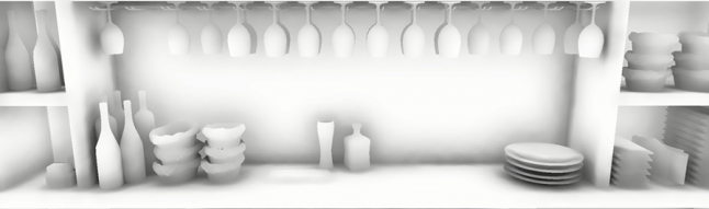
Below is the body of shader code for this pass. One extra addition, which was not mentioned before, is that we do not just pick the closest point, but rather use a probability based on barycentric coordinates to randomly pick one of three closest points. Doing this allows for a smoother transition between our discrete points, as shown in the following image. Because of the random point technique, it is also important to use neighbouring seed values, which represent neighbouring implicit voxels, as we do not know where implicit random points might reside. It is possible a random point in a neighbouring implicit voxel is closer to our world position compared to the random point generated for the current implicit voxel we reside in. To gain maximum accuracy, we iterate over all neighbouring voxels, which results in checking 27 implicit voxels.

uint GetIndexByProbability(in float3 position, in ClosestPointSample closestSamples[3])
{  
    //Create probability values based on "area" (actually just distances)
    const float3 distances = float3(
        dot(position - closestSamples[0].sample, position - closestSamples[0].sample),
        dot(position - closestSamples[1].sample, position - closestSamples[1].sample),
        dot(position - closestSamples[2].sample, position - closestSamples[2].sample));
    float3 areas = float3(
        distances[1] * distances[2],
        distances[0] * distances[2],
        distances[0] * distances[1]);
    const float totalArea = areas.x + areas.y + areas.z;
    areas /= totalArea; //normalize

    //Get random normalized value, seed based on position
    const float randomValue = randomNormalizedFloat(GetSeed(position, 15));
    
    //Get index based on probability
    return saturate(uint(randomValue / areas.x)) + saturate(uint(randomValue / (areas.x + areas.y)));
}

//Main function
ClosestPointSample GetGeneratedSample(in float3 position, in uint discreteCellSize, in uint level, 
    in uint voxelConnectivity, in uint maxLevels)
{  
    const float FLT_MAX = 3.402823466e+38f;  
    ClosestPointSample closestSamples[3];
    [unroll]
    for (int i = 0; i < 3; ++i)
    {
        closestSamples[i].sample = float3(FLT_MAX, FLT_MAX, FLT_MAX);
        closestSamples[i].seed = 0;
    }
    
    //Discretize position based on discrete cell size and current level
    const float deltaOnLevel = 1.f / (1 << level);
    const float cellSizeBasedOnLevel = discreteCellSize * deltaOnLevel;
    const float3 discretePosition = Discretize(position, cellSizeBasedOnLevel);
    
    //For that discrete position, interate over all the neighbouring voxels(based on the size of cell size)
    for (uint v = 0; v < (voxelConnectivity + 1); ++v)
    {
        //Get the offset and calculate the neighbouring absolute position
        const int3 neighbourOffsets = NeighbourOffsets[v];
        const float3 neighbourPosition = discretePosition + (neighbourOffsets * cellSizeBasedOnLevel);
        
        //Get the top level discrete position of the neighbour position. This is due to the fact 
        //that we want to find the quadrant in a normalized fashion and the fact that the neighbour 
        //position might be in the same or another voxel as the position!
        const float3 neighbourDiscreteTopPosition = Discretize(neighbourPosition, discreteCellSize);
        const float3 normalizedRelativePosition = 
            abs((neighbourDiscreteTopPosition - neighbourPosition) / (int) discreteCellSize);
        const float deltaNextLevel = deltaOnLevel * 0.5f;
        const float3 centerNormalizedRelativePosition = 
            normalizedRelativePosition + float3(deltaNextLevel, deltaNextLevel, deltaNextLevel);
        
        //Create samples in the current sub voxel & find closest!
        const float3 acp = neighbourDiscreteTopPosition 
            + (centerNormalizedRelativePosition * discreteCellSize);
        const uint absoluteSeed = GetSeedWithSignedBits(acp, maxLevels);
        
        [unroll]
        for (uint i = 0; i < 8; ++i)
        {
            uint currentSeed = absoluteSeed + i;
            uint currentLevel = level;
        
            const float3 normalizedSample = GenerateSampleInVoxelQuadrant(absoluteSeed, level, i);
            float3 absoluteSample = neighbourPosition + (normalizedSample * cellSizeBasedOnLevel);
          
            GetClosestSampleTriplet(position, absoluteSample, currentSeed, closestSamples);
        }
    }

    const uint index = GetIndexByProbability(position, closestSamples);
    return closestSamples[index];
}

Updating Data Structures

The next phase is the “Accumulation Pass”. During this pass, we simply accumulate all the shading information by using an atomic addition operation. This can change depending on your hash table implementation. A sample, based on David Farrell's implementation, can be found in the full prototype source code.

More importantly is the merging of the accumulated data and the persistent hash table. Because we are storing AO information in a range of [0, 1], we can store the shading information as a fixed-point representation where most of the bits are used for the fractional part. During the accumulation pass, this cannot be done as we potentially accumulate multiple normalized values. In other words, the fixed-point representation between both data structures is slightly different. During the merge pass, we take this into account and remap the values to the appropriate range. Finally, we also rescale the final value we store in the persistent hash table with a constant value. This is done to prevent data overflow in case a lot of AO data gets written to the same entry.

[numthreads(8, 8, 1)]
void main(uint3 DTid : SV_DispatchThreadID)
{
    const uint2 screenDimensions = uint2(1920, 1080);
    
    //Input Data
    const uint index = uint(DTid.x + (DTid.y * screenDimensions.x));
    if (index >= AccumulationHashTableElementCount)
        return;
    
    //Store in World Hash Table
    const KeyData accumulatedData = HashTableLookupBySlotID(AccumulationBuffer, 
        AccumulationHashTableElementCount, index);
    if (accumulatedData.key == 0) //No data accumulated, exit
        return;
    
    //Because no additional hashing in hashtable, the key is the seed value used
    const uint se = accumulatedData.key;
    const KeyData cachedData = HashTableLookup(WorldHashTable, WorldHashTableElementCount, se);
    
    //Perform constant rescale to prevent overflow
    const float constantOverflowMultiplier = 0.9f;
    const float scaledAccumulatedCount = accumulatedData.count * constantOverflowMultiplier;
    const float cachedCount = FromFixedPoint(cachedData.count, WorldHashTableCountFractionalBits);
    
    const float totalCount = scaledAccumulatedCount + cachedCount;
    const float cachedValueTerm = (cachedCount / totalCount) 
        * FromFixedPoint(cachedData.value, WorldHashTableValueFractionalBits);
    const float accumulationValueTerm = (scaledAccumulatedCount / totalCount) 
        * (FromFixedPoint(accumulatedData.value, AccumulationHashTableValueFractionalBits) 
            / accumulatedData.count);
    
    const uint valueToStore = ToFixedPoint(cachedValueTerm + accumulationValueTerm, 
        WorldHashTableValueFractionalBits);
    const uint countToStore = ToFixedPoint(totalCount, WorldHashTableCountFractionalBits);

    //Store in World Hash Table
    HashTableInsert(WorldHashTable, WorldHashTableElementCount, se, valueToStore, countToStore);
}

Visualization

The last phase is very similar to the code used during the implicit point generation. The main difference is that we do not look for the closest point, but instead acquire the shading information stored in each implicit point within a certain radius. When getting this data, we rescale the data based on a weight value which is determined by an inversed Euclidean distance. We thus use a modified Shepard interpolation to filter the cached shading information.

//Visualize the pixel by interpolating in world space using a modified Shepard interpolation.
//Single level as it doesn't guarantee data for previous levels.
float WorldSpaceShepardInterpolationSingleLevel(in uint discreteCellSize, in uint level,
    in float3 pixelWorldPosition, in uint maxLevels)
{
    //Shepard Interpolation Variables
    const float searchRadius = float(discreteCellSize) / float(1 << level);
    float valueSum = 0.f;
    float weightSum = 0.f;
    
    //For that discrete position, interate over all the neighbouring voxels
    //(based on the size of cell size)
    for (uint v = 0; v < (VoxelConnectivity + 1); ++v)
    {
        //Seed Generation similar to Implicit Point Generation
		//...
        for (uint i = 0; i < 8; ++i)
        {
			//...
            //Interpolation - Due to going over all points per subvoxel, duplicates are not possible
            const KeyData cachedData = 
                HashTableLookup(WorldHashTable, WorldHashTableElementCount, currentSample.seed);
            if (cachedData.key != 0)
            {
                const float sampleCount = FromFixedPoint(cachedData.count, 
                    WorldHashTableCountFractionalBits);
                const float dist = distance(pixelWorldPosition, currentSample.sample);
                const float weight = clamp(searchRadius - dist, 0.f, searchRadius) * sampleCount;
                
                valueSum += FromFixedPoint(cachedData.value, WorldHashTableValueFractionalBits) * weight;
                weightSum += weight;
            }
        }
    }
    
    if (weightSum > 0)
        valueSum /= weightSum;
    
    return valueSum;
}

Results & Future Work

Using this technique, we effectively combine the idea of 3D random point sets with a simpler representation in memory. Because the data is stored in world space, the data can be used as is. Below you can see a working example, where we temporarily pause the accumulation to showcase that data is effectively stored and filtered in world space.

While there is still room for a lot of improvements (e.g. adaptive point density based on level of detail or local shading complexity, variable update rates, support of dynamic changes using temporal integration based on exponential moving averages, etc.), the first results are interesting. In our research, we compared our results with a partial implementation of Nvidia’s path space filtering technique. The metrics, results, our findings and more overall details can be found in the thesis.

For any questions, remarks or suggestions, feel free to reach out to the author.

Bibliography

J. T. Kajiya, “The rendering equation,” Proc. 13th Annu. Conf. Comput. Graph. Interact. Tech. SIGGRAPH 1986, vol. 20, no. 4, pp. 143–150, 1986, doi: 10.1145/15922.15902.
P. H. Christensen, “Point-Based Global Illumination for Movie Production,” no. July, 2010.
T. Stachwiak, “Stochastic all the things: Raytracing in hybrid real-time rendering,” Digital Dragons, 2018. https://www.ea.com/seed/news/seed-dd18-presentation-slides-raytracing (accessed Oct. 29, 2020).
A. Keller, K. Dahm, and N. Binder, “Path space filtering,” ACM SIGGRAPH 2014 Talks, SIGGRAPH 2014, pp. 1–12, 2014, doi: 10.1145/2614106.2614149.
N. Binder, S. Fricke, and A. Keller, “Massively Parallel Path Space Filtering,” 2019, [Online]. Available: http://arxiv.org/abs/1902.05942.
SHEPARD D, “Two- dimensional interpolation function for irregularly- spaced data,” Proc 23rd Nat Conf, pp. 517–524, 1968.
M. Jarzynski and M. Olano, “Hash Functions for GPU Rendering,” J. Comput. Graph. Tech. Hash Funct. GPU Render., vol. 9, no. 3, pp. 20–38, 2020, [Online]. Available: http://jcgt.orghttp//jcgt.org.
P. Christensen, A. Kensler, and C. Kilpatrick, “Progressive Multi-Jittered Sample Sequences,” Comput. Graph. Forum, vol. 37, no. 4, pp. 21–33, 2018, doi: 10.1111/cgf.13472.
Read more about:
Featured BlogsAbout the Author(s)
You May Also Like
.jpeg?width=700&auto=webp&quality=80&disable=upscale)