GDC 2002: Incredibly Dense Meshes

This paper proposes a general solution for a problem that will probably arise in the near future, perhaps with the launch of PlayStation 3 and its counterparts. Presupposed is the exacerbation of a current trend in console hardware, where hardware transformation, lighting, and triangle drawing outpace the hardware's capacity to store and move data. In other words, in the future, transforming vertices and drawing triangles will be virtually free in comparison with storing model data and reading it from main RAM.

For brevity the paper focuses on a solution for character models. On the one hand, character models pose more problems than fixed environment geometry in regard to controlling the animation of vertices with bones. On the other hand, culling and view-dependent level-of-detail need not be considered.

The summary of the problem we propose to solve is as follows: render a very dense animated skinned character mesh in "the future," when transforming vertices and drawing triangles will be cheap, and when loading from RAM will be expensive. (For programmers of the PS2, this "future" will sound more like the present!)

The contribution of this paper is to collect together several already-published conceptions and propose their application to the problem at hand. Some details are given here, but the reader is encouraged to consult the academic papers in the References for more detail.

Later sections discusse the details of the problem, outline several techniques whose integration yields a potential solution, and briefly discuss a possible future without textures.

The Future of Character Models

With the onset of the next "new thing" in game hardware, consumer expectation could very well be an amount of detail equivalent to one triangle per pixel. If screen resolution continues to double with each generation, 1024x768 will be the typical screen size. If, when close to the view, a character model occupies roughly 50% of the screen pixels, and given that the model has half its triangles facing away from the view, then the total triangle count will be nearly 800,000 triangles per character model.

Will transformation and drawing performance really be up to this task? To answer that question, let's look at the advance we saw from PS1 to PS2. The best PS1 character engines seen by the author could render about 20 400-triangle characters at 30Hz, with only single-bone control and no dynamic lighting. The author has seen character engines on PS2 with performance of 31 3400-triangle characters at 60Hz, with up to 3 bones per vertex and with dynamic lighting on all vertices. Even ignoring the added bone control and the dynamic lighting, we have an increase by a factor of more than 25.

So let's assume that transformation and drawing performance will increase again by a factor of 25. In terms of total capacity for a character renderer, PS3 will then have the ability to transform, light, and draw 31*3400*25 > 2.6 million triangles per frame at 60Hz.

If we have a system incorporated LOD control, if we assume the 800,000-triangle density above, and if on average each character occupies only 25% of its near-view screen space, then we would have to render an average of 200,000 triangles per character. This means that in games like team sports, where most of the rendering horsepower is devoted to character rendering, it is perfectly reasonable that we'll be seeing 10 characters in a scene where at maximum detail, each character is 800,000 triangles.

Make the following assumptions about storage technique:

• Indexed triangle strips. Each strip vertex has a 32-bit index and 32-bit texture coordinates (16-bits for U and for V).
  
• Each vertex is 32-bit floating-point.
  
• The mesh has a 2-to-1 triangle-to-vertex ratio.
  
• Stripping performance is 8 strip vertices per strip.
  

With these assumptions, current techniques will result in the following storage needs for each character:

So for the characters in our 10-character scene, we would need to store 83MB of data and mess with it each frame.

While predicting the future is dangerous, it is the author's opinion that future hardware will be able to easily transform and draw meshes of the above size but that it will not be able to store and access that much data. The predicted implications are that rendering techniques that store and move only small amounts of data will be necessary in order to meet consumer expectations of visual quality. Those rendering techniques will have to include smooth LOD control.

Loop Subdivision Surfaces

Loop Subdivision Surfaces provide a solution to the problems predicted above by having the following advantages:

• The program need store only a course base mesh with which an algorithm procedurally generates a smooth surface.
  
• The vertices of the base mesh can be animated with bone control, still allowing the rendered mesh to be created procedurally.
  
• Smooth LOD control is implicit in the method as a result of blending between 2 levels of subdivision.
  
• Sharp edges can be included with continuous sharpness control.
  
• Base meshes of any topology can be used.
  

The Basics
This section gives a very brief explanation of how Loop Subdivision works. For a full exposition of subdivision surfaces, see [7].

Begin with a base mesh. The base mesh data structure must have triangles, edges, and vertices. The vertices store the actual geometry and color content for the model. All features (vertices, edges, triangles) must store information on the connectivity to other features. The exact format of this connectivity depends on the rendering method. To help explain the Loop scheme below, we will use a naïve structure for vertices as follows. For simplicity the structure stores only geometric position and not color information.

  typedef struct
  {
     VERT* parents[2]; // Verts on birth edge.
     VERT* across[2]; // Verts opposite birth edge.
     ARRAY<VERT*> adjs; // Vertices sharing an edge.
     VECTOR pos;
     VECTOR normal;
  } VERT;

The "parents" are the vertices of the "birth" edge from which the vertex was originally created in the splitting step. The "across" are the vertices opposite the birth edge. The "adjs" are the vertices sharing an edge with the vertex. In the subdivision algorithm, "parents" and "across" are used only in the first average when the vertex is created from a split. The "adjs" are used only in subsequent averages. Figure 1 illustrates the VERT structure. Note that the "adjs" must be stored in counter-clockwise order for the tangent computation to work properly.

Rendering a subdivided mesh consists of a recursive process where at each level of recursion there are two steps. The first step is the splitting step, where the mesh is each triangle is split into 4 triangles at the midpoints of each edge. The second step is the averaging step, where the positions of each vertex in the split mesh are perturbed according to a weighted average of neighboring vertices.

For Loop Subdivision there are four cases for the averaging rules. At each level of subdivision, there are two kinds of vertices: the vertices that were already there ("old"), and the vertices that were just created by the split ("new"). For both old and new vertices, boundary vertices, or vertices that lie touching an edge with only one adjacent triangle, are handled differently from interior vertices.
After the entire mesh is subdivided and averaged, then the result can be passed back into the algorithm and subdivided again. Repeating this process produces nice smooth meshes.
The logic for averaging a single vertex of the mesh is given in the code below.

  void ComputeAverage(VERT* vert) {
    if(Vertex_Created_By_Split(vert)) {
      VERT* par0 = vert->parents[0];
      VERT* par1 = vert->parents[1];
      VERT* acc0 = vert->across[0];
      VERT* acc1 = vert->across[1];

      if(Vertex_On_Boundary(vert)) {
        vert->pos = (par0->pos+par1->pos)/2;
      }
      else {
            vert->pos = (3.0/8.0)*par0->pos+
            (3.0/8.0)*par1->pos+
            (1.0/8.0)*acc0->pos+
            (1.0/8.0)*acc1->pos;
      }
    }
    else {
          if(Vertex_On_Boundary(vert)) {
            vert->pos = (6.0/8.0)*vert->pos;
            for(int i=0;i<vert->adjs.Size();i++) {
              // Exactly 2 should be on boundary.
              VERT* a = vert->adjs[i];
              if(Vertex_On_Boundary(a)) {
                  vert->pos += (1.0/8.0)*a->pos;
               }
          }
      }
      else {
            int n = adjs.Size();
            float temp = 3 + 2*cos(2.0*PI/n);
            float alpha = (40.0 - temp*temp) / 64.0;
            vert->pos = (1-alpha)*vert->pos;
            alpha /= n;
            for(int i=0;i<n;i++) {
               vert->pos += alpha * vert->adjs[i]->pos;
            }
         }
      }
   }

Visual representations in so-called "Averaging Masks" can been seen in virtually every paper on subdivision surfaces.

Edge Sharpness
What if you want some sharp edges? Edge sharpness is an area where subdivision surfaces have an advantage over Bezier patches and NURBs, because it is easy to control the degree of sharpness at an edge.

To make an edge look sharp, we simple skip the averaging step for any vertices on the edge. The program can set the degree of sharpness by how many levels of subdivision it waits before applying the averaging step again. See [3] for details and examples.

Normal Offsets
While a subdivision surface will be nice looking and very smooth, there are always needs for finer detail. The program can add this fine detail with normal offsets, or "displacements" as [4] calls them.

Just as vertex positions can be computed procedurally weighted averages of neighboring vertices, tangents at those vertex positions can be computed as well. Two non-parallel tangents can be computed, and their outer product may be taken, producing a normal to the surface at the vertex. The logic for computing two tangent vectors is given in the following code. See [7] for an exposition of how this computation is derived.

  void ComputeNormal(VERT* vert) {
     int n = vert->adjs.Size();
     VECTOR tang_a(0,0,0);
     VECTOR tang_b(0,0,0);
     for(int i=0;i<n;i++) {
        float temp = 2*i*PI/n;
        float s = sin(temp);
        float c = cos(temp);
        tang_a += vert->adjs[i]->pos * s;
        tang_b += vert->adjs[i]->pos * c;
     }

     vert->normal = OuterProduct(tang_a,tang_b);
  }

Once the normal at a vertex is computed, its final position is just a scalar displacement value multiplied by that normal. Note that for smooth shading, the normal at the displaced vertex may be needed. This displaced vertex normal is not the same as the subdivision surface normal, and its computation is a bit trickier. See [4] for more detail.

Color Offsets
Just as geometric coordinates can be stored as part of the vertex data, additional "scalar fields," as [3] calls them, can be included for vertex colors. Just as normal offsets can be added to displace the vertices, color offsets can be added to the subdivided color values.

Color offsets create a framework for a character model that doesn't require textures. Given that our supposed triangle size is one triangle per pixel anyway, textures start to seem impractical, especially on character models where there is little opportunity to repeat or tile textures.
When used along with the Wavelet Compression described below, color offsets to the results of color subdivision as scalar fields provide a practical and more flexible alternative to texture mapping.

Real-Time Rendering?
Naively implementing Loop Subdivision as a recursive process is prohibitively slow and would not be appropriate for a game display engine. In recent years, however, numerous techniques ([1], [2], [6]) for rendering with the Loop scheme have been proposed and implemented.

Wavelet Compression

If we want the added data of normal displacements and color offsets, we're going to have to compress it somehow for the data size to be practical. Because of their similarity regarding weighted averages, wavelet compression techniques are well suited to the task.

Without getting into the mathematics of wavelets, the basic idea behind their use for compression is that data can be reduced in size, with minimal loss of fidelity, if it first transformed into a set of averages and a set of details rather than in it's original form. In a similar approach to creating a subdivision surface, a program will average two or more data points (vertices if you will), storing not just the average but also the difference between the data points and the average. The process is then repeated, this time only on the just-created averages. When complete, the data stream will be the same size as the original, beginning with one overall average followed by difference, or "detail" points.

If the averaging scheme has certain properties, the resulting data will be such that if the smallest of the detail points are turned to zero, and if the transformation is inverted, the result of the inverted process will be very close to the original.

Compression is achieved after turning small values to zero and then storing the data in a runs-of-zeros scheme.

Harr Wavelets
The simplest of the wavelet schemes is the Harr Wavelet scheme, defined over a 1-dimensional set of points. The following code will make a single pass on a set of floating-point numbers, performing a transformation according to the Harr Scheme. Each successive pair of numbers is simply summed and then multiplied by a scalar, 1.0/sqrt(2). The scalar multiplication is to maintain normalization, discussed later.

  void Harr(float* input,float* output,int size)
  {
     int half = size >> 1;
     float scale = 1.0f / (float)sqrt(2.0f);
     for(int i=0;i<half;i++) {
        float i0 = input[(i<<1)+0];
        float i1 = input[(i<<1)+1];
        output[i] = (i0+i1) * scale;
        output[i+half] = (i0-i1) * scale;
     }
  }

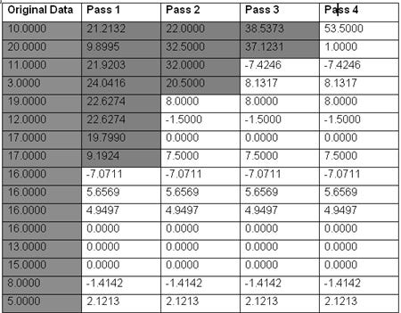
The table below gives example data acted upon by the routine above. Note the following:

• In each pass, the "averages" are placed in the beginning of the data, and the "details" are placed at the end.
  
• Each pass acts on half the amount of data of the previous pass.
  
• The first entry in Pass 4, 53.5, is the sum of the original data divided by sqrt(2)^4, or in other words, a scaled overall average of the original data.
  
• In practice, the data streams must be fairly large in order to see any dramatic reduction by throwing out small values.
  

Generalization Using Matrices
The code in the last section can be generalized into matrix form as follows. For brevity, we will show the matrix form of Pass 3 from the table above.

In this context, the first two rows in the above matrix, the ones that create the averages, correspond to the "scaling functions" referred to in the literature, which in the case of Harr wavelets are just 1-D step-functions. The second two rows, the ones that create the details, correspond to what are called the "wavelets" in the literature.

"Almost" Wavelets as Opposed to True Wavelets
Harr is one of the few wavelet schemes that is both practical and uses true wavelets. The most elusive condition that must be satisfied in order to be a true wavelet scheme is the condition that the wavelets be orthogonal to the scaling functions and orthogonal to each other. By taking the inner products of the rows in the matrix of it is clear that under the Harr scheme is indeed orthogonal. In the general case, however, especially when it comes to schemes applied to 3D geometry, the orthogonality condition must be lifted. The math community has coined a few new terms, like semi-orthogonal and bi-orthogonal, which basically mean that the resulting schemes are "almost" wavelets J. The text in [5] goes into detail on this issue.

Another important attribute of a wavelet scheme is normalization. Recall in the routine of Harr wavelets section that each average is weighted by a factor of 2/sqrt(2), implemented by summing the terms and dividing by sqrt(2). This is done so that successive averaging and differencing do not in appropriately scale the later passes. Normalization is done so that the relative size of elements after the final pass gives an accurate indication of how important they are to the data so that error tolerances will have their usual meaning.

Loop Subdivision as a Wavelet Scheme

There are actually two purposes in applying a wavelet-like solution to compressing the color offsets and normal displacements of our subdivision surface. The first is compression. The second is to allow editing of the model at different levels of resolution.

Note that while advocating the techniques of [5], this paper proposes them for a slightly different use. While sharing the topological aspects of [5], the actual data we want to compress is slightly different. Whereas [5] aims to allow a mesh to be parameterized as a subdivision surface and stored using wavelets, we propose using the same technique only to compress normal displacements and color offsets, not an arbitrary original mesh.

Matrix Construction
At each level of subdivision, there are two matrices that need construction. The first is the analysis matrix, which transforms the color offsets and normal displacements from their values in the higher level to weighted averages and detail coefficients in their lower level. The second matrix is the synthesis matrix, which performs the opposite task as the analysis matrix, and in fact is just the matrix inverse of the analysis matrix.

Full details of how to construct these matrices are beyond the scope of this paper, and they have already been laid out with examples in [5]. The serious reader should definitely read [5] before building a system combining subdivision surfaces and wavelets.

To summarize matrix construction of [5], the synthesis matrix is constructed first, and the analysis matrix is computed as the synthesis matrix's inverse. Suppose that in the current level of subdivision we are going from M vertices up to N (greater than M) vertices. In block form, the synthesis matrix is given by [P Q], where P is an N x M matrix and Q is an N x (N-M) matrix. Construction of P is very simple, just consisting of rows whose columns contain the same coefficients that the subdivision surface scheme uses to average vertices when going to the next subdivision level (see the code in section 3.1). The complexity is in the construction of the Q matrix. Patient reading of [5] will yield an understanding of how to compute Q for any subdivision scheme, not just the Loop scheme.

Sparse Matrices
Actually implementing the technique with naïve N-by-N matrices is of course not recommended, because the size of these matrices would be ridiculously large. Instead, either the process should simply be coded in direct fashion, or at a minimum sparse matrix classes should be employed.

Is the Synthesis Matrix Invertible?
In [5] there is no explicit statement that the synthesis matrix [P Q] is invertible. The reader may wonder if there can be a case where the analysis matrix cannot be produced by inversion. Without diving too far into the details of [5], it is relevant [5] shows [P Q] to be of the following block form:

In this form, O are the rows corresponding to the vertices already a part of the lower level of subdivision, N are the rows corresponding to the vertices created by the splits, and a is a special "magic" matrix derived in [5]. Although not explicitly clear, a section in [5] regarding the whether O is invertible for primal schemes (Loop is a primal scheme) implies that O is invertible for Loop. The text in [5] states that most primal schemes have invertible O, with Catmull-Clark as the only noted exception. Therefore we aim to show here only that if O is invertible, then so is [P Q].

It can be shown easily through block matrix multiplication that the inverse of [P Q] as given above is as follows:

(Inv(O) means the inverse of O.) Therefore if O is invertible, so is [P Q].

What about Textures?

Part of the author's view of the future is that eventually we will stop using those annoying textures. Compressing them, transferring them about, dealing with caching, etc., etc., are horrid nuisances that become obviated once meshes get very dense, especially for characters where there is little opportunity to repeat textures anyway. The author hopes for a time when character models are simply painted on their surfaces by an artist.

Naturally the storage of all that color data would be prohibitive for an 800,000-triangle mesh, but by efficiently implementing the techniques outlined here and detailed in the references, perhaps a texture-less world can become a reality. Barring that, [2] gives a practical method for incorporating "texture meshes" into the scheme, whereby the connectivity of the texture coordinates is handled separately but in similar fashion to the geometry.

Conclusion
Industrial use of subdivision surfaces in real-time has yet to gain much of a following, at least within the game business. Graphic quality in games is still only on the cusp of requiring curved surface techniques at all. Furthermore, while [1], [2], and [6] implement viable methods for rendering subdivision surfaces in real-time, the problems of efficiently combining the techniques outlined in this paper remain open. In particular, synthesizing the color offsets and normal displacements from their compressed form in a manner compatible with small-cache graphics hardware will be very challenging. Hopefully a unified, efficient implementation scheme will be available before the onset of the next "Next Gen" hardware.

References

[1] Bischoff, "Towards Hardware Implementation of Loop Subdivision", Proceedings 2000 SIGGRAPH/EUROGRAPHICS Workshop on Graphics Hardware, August 2000.

[2] Brickhill, "Practical Implementation Techniques for Multi-Resolution Subdivision Surfaces". GDC Conference Proceeding, 2001.

[3] DeRose, "Subdivision Surfaces in Character Animation". Proceedings of the 25th annual conference on Computer Graphics, 1998, Pages 85 - 94.

[4] Hoppe, "Displaced Subdivision Surfaces". Computer Graphics Proceedings, SIGGRAPH 2000, 2000.

[5] Lounsbery, "Multiresolution Analysis for Surfaces of Arbitrary Topological Type". ACM Transactions on Graphics, Vol. 16, No. 1, January 1997, Pages 34-73.

[6] Pulli, "Fast Rendering of Subdivision Surfaces". The art and interdisciplinary programs of SIGGRAPH '96 on SIGGRAPH '96 visual proceedings, 1996, Page 144.

[7] Zorin, "Subdivision for Modeling and Animation". SIGGRAPH '98 Course Notes, 1998. http://www.multires.caltech.edu/teaching/courses/subdivision