Toward More Realistic Pathfinding

Pathfinding is a core component of most games today. Characters, animals, and vehicles all move in some goal-directed manner, and the program must be able to identify a good path from an origin to a goal, which both avoids obstacles and is the most efficient way of getting to the destination. The best-known algorithm for achieving this is the A* search (pronounced "A star"), and it is typical for a lead programmer on a project simply to say, "We'll use A* for pathfinding." However, AI programmers have found again and again that the basic A* algorithm can be woefully inadequate for achieving the kind of realistic movement they require in their games.

This article focuses on several techniques for achieving more realistic looking results from pathfinding. Many of the techniques discussed here were used in the development of Activision's upcoming Big Game Hunter 5, which made for startlingly more realistic and visually interesting movement for the various animals in the game. The focal topics presented here include:

Dealing with realistic turns is an important and timely AI topic. In the August 2000 issue of Game Developer ("The Future of Game AI"), author Dave Pottinger states, "So far, no one has proffered a simple solution for pathing in true 3D while taking into account such things as turn radius and other movement restrictions," and goes on to describe some of the "fakes" that are commonly done. Also, in a recent interview on Feedmag.com with Will Wright, creator of The Sims, Wright describes movement of The Sims' characters: "They might have to turn around and they kind of get cornered -- they actually have to calculate how quickly they can turn that angle. Then they actually calculate the angle of displacement from step to step. Most people don't realize how complex this stuff is..."

In addition to the above points, I will also cover some important optimization techniques, as well as some other path-related topics such as speed restrictions, realistic people movement, and movement along roads. After presenting the various techniques below, we'll see by the end that there is no true "best approach," and that the method you choose will depend on the specific nature of your game, its characters, available CPU cycles and other factors.

Note that in the world of pathfinding, the term "unit" is used to represent any on-screen mobile element, whether it's a player character, animal, monster, ship, vehicle, infantry unit, and so on. Note also that while the body of this article presents examples based on tile-based searching, most of the techniques presented here are equally applicable to other types of world division, such as convex polygons and 3D navigation meshes.

A Brief Introduction to A*

The A* algorithm is a venerable technique which was originally applied to various mathematical problems and was adapted to pathfinding during the early years of artificial intelligence research. The basic algorithm, when applied to a grid-based pathfinding problem, is as follows: Start at the initial position (node) and place it on the Open list, along with its estimated cost to the destination, which is determined by a heuristic. The heuristic is often just the geometric distance between two nodes. Then perform the following loop while the Open list is nonempty:

In the end, the nodes along the chosen path, including the starting and ending position, are called the waypoints. The A* algorithm is guaranteed to find the best path from the origin to the destination, if one exists. A more detailed introduction to A* is presented in Bryan Stout's Game Developer article "Smart Moves: Intelligent Pathfinding" (October/November 1996), which is also available on Gamasutra.com.

Hierarchical Pathfinding

Critical to any discussion of efficient pathfinding within a game is the notion of hierarchical maps. To perform an efficient A* search, it is important that the origin and destination nodes of any particular search are not too far apart, or the search time will become enormous. I recommend that the distance between origin and destination be constrained to 40 tiles, and that the total search space be no more than 60x60 tiles (creating a 10-tile-wide buffer behind both origin and destination, allowing the path to wrap around large obstacles.) If units need to search for more distant destinations, some method of hierarchical pathfinding should be used.

In the real world, people do not formulate precise path plans which stretch on for miles. Rather, if a person has some domain knowledge of the intermediate terrain, they will subdivide the path, i.e. "first get to the highway on-ramp, then travel to the exit for the mall, then drive to the parking lot." Alternatively, if a person has no domain knowledge, they will create intermediate points as they see them. For example, if you wanted to eventually reach some point you knew was far to the North, you would first look North and pick a point you could see, plan a path toward it, and only when you got there, you would pick your next point.

Within a game program, the techniques for creating a map hierarchy include:

A Faster Implementation of the Standard A*

Before proceeding with turning and smoothing modifications to the A* algorithm, let's start with some basic optimizations that can speed up the standard A* algorithm by a factor of 40 or more. To start with, the standard A* algorithm uses a sorted linked list (or two linked lists) to track nodes that are checked. Instead, we'll use a 60x60 fixed matrix. When starting a search from point a to point b, we find the midpoint between those two and place it at point [30,30] on our matrix. Each point on the matrix stores:

We also keep a separate array of 1-bit Booleans, which store whether or not each node in our matrix has been touched yet during this search. That way, we can very rapidly initialize at the beginning of the search without needing to clear the entire matrix.

Whereas the original algorithm maintains a separate sorted Open list (actually a Priority Queue), we instead maintain basic list functionality simply by using Previous and Next pointers within the fixed array. Note that we do have the memory requirement for our 60x60 matrix, but our compacted data structure requires only 16 bytes per node, for a total of 57K. (Even expanding the matrix to 120x120 will only require 230K of memory.)

Note additionally that the "list" can be implemented as a binary tree (by having two Next node pointers at each element), but we've actually found it to be substantially faster to have a simple (non-priority) list. While this does result in time O(n) for the search for the lowest cost node at the top of the A* loop (rather than O(log n) for a priority queue), it excels in that all insertions and deletions, of which there are many, are only O(1). Best of all, it eliminates the inner loop search that checks if neighboring nodes yet exist on the Open or Closed lists, which otherwise would take O(n) (or maybe a bit better if a hash table is used).

Overall, by avoiding all memory allocations and list insertions, this method turns out to be dramatically faster. I have profiled it to be as much as 40 times faster than standard A* implementations.

Note that for the Directional search described later in this article, eight times the number of nodes are necessary, so the memory requirement will all increase by a factor of eight.

Smoothing the A* Path

The first and most basic step in making an A* path more realistic is getting rid of the zigzag effect it produces, which you can see in Figure 2a. This effect is caused by the fact that the standard A* algorithm searches the eight tiles surrounding a tile, and then proceeds to the next tile. This is fine in primitive games where units simply hop from tile to tile, but is unacceptable for the smooth movement required in most games today.

One simple method of reducing the number of turns is to make the following modification to the A* algorithm: Add a cost penalty each time a turn is taken. This will favor paths which are the same distance, but take fewer turns, as shown in Figure 2b. Unfortunately, this simplistic solution is not very effective, because all turns are still at 45-degree angles, which causes the movement to continue to look rather unrealistic. In addition, the 45-degree-angle turns often cause paths to be much longer than they have to be. Finally, this solution may add significantly to the time required to perform the A* algorithm.

The actual desired path is that shown in Figure 2c, which takes the most direct route, regardless of the angle. In order to achieve this effect, we introduce a simple smoothing algorithm which takes place after the standard A* algorithm has completed its path. The algorithm makes use of a function Walkable(pointA, pointB), which samples points along a line from point A to point B at a certain granularity (typically we use one-fifth of a tile width), checking at each point whether the unit overlaps any neighboring blocked tile. (Using the width of the unit, it checks the four points in a diamond pattern around the unit's center.) The function returns true if it encounters no blocked tiles and false otherwise. See Figure 3 for an illustration, and Listing 1 for pseudocode.

LISTING 1. Pseudocode for the simple smoothing algorithm. The smoothing algorithm simply checks from waypoint to waypoint along the path, trying to eliminate intermediate waypoints when possible.

checkPoint = starting point of path
currentPoint = next point in path
while (currentPoint->next != NULL)
if Walkable(checkPoint, currentPoint->next)
// Make a straight path between those points:
temp = currentPoint
currentPoint = currentPoint->next
delete temp from the path
else
checkPoint = currentPoint
currentPoint = currentPoint->next

The smoothing algorithm simply checks from waypoint to waypoint along the path, trying to eliminate intermediate waypoints when possible. To achieve the path shown in Figure 2c, the four waypoints shown in red in Figure 2a were eliminated.

Since the standard A* algorithm searches the surrounding eight tiles at every node, there are times when it returns a path which is impossible, as shown with the green path in Figure 4. In these cases, the smoothing algorithm presented above will smooth the portions it can (shown in purple), and leave the "impossible" sections as is.

This simple smoothing algorithm is similar to "line of sight" smoothing, in which all waypoints are progressively skipped until the last one that can be "seen" from the current position. However, the algorithm presented here is more accurate, because it adds collision detection based on the width of the character and also can be used easily in conjunction with the realistic turning methods described in the next section.

Note that the simple smoothing algorithm presented above, like other simple smoothing methods, is less effective with large units and with certain configurations of blocking objects. A more sophisticated smoothing pass will be presented later.

Adding Realistic Turns

The next step is to add realistic curved turns for our units, so that they don't appear to change direction abruptly every time they need to turn. A simple solution involves using a spline to smooth the abrupt corners into turns. While this solves some of the aesthetic concerns, it still results in physically very unrealistic movement for most units. For example, it might change an abrupt cornering of a tank into a tight curve, but the curved turn would still be much tighter than the tank could actually perform.

For a better solution, the first thing we need to know is the turning radius for our unit. Turning radius is a fairly simple concept: if you're in a big parking lot in your car, and turn the wheel to the left as far as it will go and proceed to drive in a circle, the radius of that circle is your turning radius. The turning radius of a Volkswagen Beetle will be substantially smaller than that of a big SUV, and the turning radius of a person will be substantially less than that of a large, lumbering bear.

Let's say you're at some point (origin) and pointed in a certain direction, and you need to get to some other point (destination), as illustrated in Figure 5. The shortest path is found either by turning left as far as you can, going in a circle until you are directly pointed at the destination, and then proceeding forward, or by turning right and doing the same thing.

In Figure 5 the shortest route is clearly the green line at the bottom. This path turns out to be fairly straightforward to calculate due to some geometric relationships, illustrated in Figure 6.

First we calculate the location of point P, which is the center of our turning circle, and is always radius r away from the starting point. If we are turning right from our initial direction, that means P is at an angle of (initial_direction - 90) from the origin, so:

angleToP = initial_direction - 90
P.x = Origin.x + r * cos(angleToP)
P.y = Origin.y + r * sin(angleToP)

Now that we know the location of the center point P, we can calculate the distance from P to the destination, shown as h on the diagram:

dx = Destination.x - P.x
dy = Destination.y - P.y
h = sqrt(dx*dx + dy*dy)

At this point we also want to check that the destination is not within the circle, because if it were, we could never reach it:

if (h < r)
return false

Now we can calculate the length of segment d, since we already know the lengths of the other two sides of the right triangle, namely h and r. We can also determine angle from the right-triangle relationship:

d = sqrt(h*h - r*r)
theta = arccos(r / h)

Finally, to figure out the point Q at which to leave the circle and start on the straight line, we need to know the total angle + , and is easily determined as the angle from P to the destination:

phi = arctan(dy / dx) [offset to the correct quadrant]
Q.x = P.x + r * cos(phi + theta)
Q.y = P.y + r * sin(phi + theta)

The above calculations represent the right-turning path. The left-hand path can be calculated in exactly the same way, except that we add 90 to initial_direction for calculating angleToP, and later we use - instead of + . After calculating both, we simply see which path is shorter and use that one.

In our implementation of this algorithm and the ones that follow, we utilize a data structure which stores up to four distinct "line segments," each one being either straight or curved. For the curved paths described here, there are only two segments used: an arc followed by a straight line. The data structure contains members which specify whether the segment is an arc or a straight line, the length of the segment, and its starting position. If the segment is a straight line, the data structure also specifies the angle; for arcs, it specifies the center of the circle, the starting angle on the circle, and the total radians covered by the arc.

Once we have calculated the curved path necessary to get between two points, we can easily calculate our position and direction at any given instant in time, as shown in Listing 2.

LISTING 2. Calculating the position and orientation at a particular time.

distance = unit_speed * elapsed_time
loop i = 0 to 3:
if (distance < LineSegment[i].length)
// Unit is somewhere on this line segment
if LineSegment[i] is an arc
determine current angle on arc (theta) by adding or
subtracting (distance / r) to the starting angle
depending on whether turning to the left or right
position.x = LineSegment[i].center.x + r*cos(theta)
position.y = LineSegment[i].center.y + r*sin(theta)
determine current direction (direction) by adding or
subtracting 90 to theta, depending on left/right
else
position.x = LineSegment[i].start.x
+ distance * cos(LineSegment[i].line_angle)
position.y = LineSegment[i].start.y
+ distance * sin(LineSegment[i].line_angle)
direction = theta
break out of loop
else
distance = distance - LineSegment[i].length

Legal Turns: The Basic Methods

So nowthat we know how to find and follow an efficient curved line between two points, how do we use this in our pathing? The methods discussed in this section are all postprocessing techniques. In other words, they involve using the standard A* algorithm during initial pathfinding, and then adding curved turns later in some fashion, either in an extended pathfinding or during actual unit movement.

This solution is actually quite acceptable for many games. However, we often don't want to allow any obviously illegal turns where the unit overlaps obstacles. The next three methods address this problem.

Legal Turns: The Directional A* Algorithm

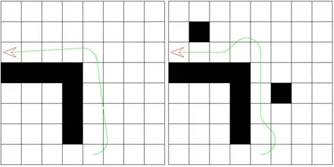
None of the methods presented in the above section is formally correct. Method two can often fail to find valid paths, and methods one, three, and four are all basically cheats. Comparing Figures 1c and 1d, we see that the only valid solution which takes turning radius into account may require a completely different route from what the basic A* algorithm provides. To solve this problem, I'll introduce a significant modification to the algorithm, which I'll term the Directional A*.

The main change to the algorithm is the addition of a third dimension. Instead of having a flat grid of nodes, where each node represents an XY grid position, we now have a three-dimensional space of nodes, where a node represents the position at that node, as well as the compass orientation of the unit (N, S, E, W, NE, NW, SE, SW.) For example, a node might be [X = 92, Y = 142, orientation = NW]. Thus there are eight times as many nodes as before. There are also 64 times as many ways of getting from one location to another, because you can start at the first node pointing any one of eight directions, and end at the next node pointing any one of eight directions.

During the algorithm, when we're at a parent node p and checking a child node q, we don't just check if the child itself is a blocked tile. We check if a curved path from p to q is possible (taking into account the orientation at p, the orientation at q, and the turning radius); and if so, we check if traveling on that path would hit any blocked tiles. Only then do we consider a child node to be valid. In this fashion, every path we look at will be legal, and we will end up with a valid path given the size and turning radius of the unit. Figure 8 illustrates this.

The shortest path, and the one that would be chosen by the standard A* algorithm, goes from a to c. However, the turning radius of the unit prevents the unit from performing the right turn at c given the surrounding blockers, and thus the standard A* would return an invalid path in this case. The Directional A*, on the other hand, sees this and instead looks at the alternate path through b. Yet even at b, a 90 degrees turn to the left is not possible due to nearby blockers, so the algorithm finds that it can make a right-hand loop and then continue.

Directional Curved Paths

In order to implement the Directional A* algorithm, it is necessary to figure out how to compute the shortest path from a point p to a point q, taking into account not only starting direction, orientation, and turning radius, but also the ending direction. This algorithm will allow us to compute the shortest legal method of getting from a current position and orientation on the map to the next waypoint, and also to be facing a certain direction upon arriving there.

Earlier we saw how to compute the shortest path given just a starting orientation and turning radius. Adding a fixed final orientation makes the process a bit more challenging.

There are four possible shortest paths for getting from origin to destination with fixed starting and ending directions. This is illustrated in Figure 9. The main difference between this and Figure 5 is that we approach the destination point by going around an arc of a circle, so that we will end up pointing in the correct direction. Similar to before, we will use trigonometric relationships to figure out the angles and lengths for each segment, except that there are now three segments in total: the first arc, the line in the middle, and the second arc.

We can easily position the turning circles for both origin and destination in the same way that we did earlier for Figure 6. The challenge is finding the point (and angle) where the path leaves the first circle, and later where it hits the second circle. There are two main cases that we need to consider. First, there is the case where we are traveling around both circles in the same direction, for example clockwise and clockwise (see Figure 10).

For this case, note the following:

The second case, where the path travels around the circles in opposite directions (for example, clockwise around the first and counterclockwise around the second), is somewhat more complicated (see Figure 11). To solve this problem, we imagine a third circle centered at P3 which is tangent to the destination circle, and whose angle relative to the destination circle is at right angles with the (green) path line. Now we follow these steps:

We now know how to determine all four paths from origin to destination, so given two nodes (and their associated positions and directions), we can calculate the four possible paths and use the one which is the shortest.

Note that we can now use the simple smoothing algorithm presented earlier with curved paths, with just a slight modification to the Walkable(pointA, pointB) function. Instead of point-sampling in a straight line between pointA and pointB, the new Walkable(pointA, directionA, pointB, directionB) function samples intermediate points along a valid curve between A and B given the initial and final directions.

Discrete and nondiscrete positions and directions. Some readers may be concerned at this point, since it seems that our algorithm is dependent on movement always starting at exactly the center position of a tile, and at exactly one of eight compass directions. In real games, a character may be in the middle of walking between two tiles at the exact moment we need it to change direction. In fact, we can easily modify the algorithm so that whenever the origin node is the starting point of the search, we do the curve computations based on the true precise position and angle of the character's starting point. This eliminates the restriction.

Nonetheless, the algorithm still requires that the waypoints are at the center of tiles and at exact compass directions. These restrictions can seemingly cause problems where a valid path may not be found. The case of tile-centering is discussed in more detail below. The problem of rounded compass directions, however, is in fact very minimal and will almost never restrict a valid path. It may cause visible turns to be a bit more exaggerated, but this effect is very slight.

Expanded searching to surrounding tiles. So far in this discussion, we have assumed that at every node, you check the surrounding eight locations as neighbors. We call this a Directional-8 search. As mentioned in the preceding paragraph, there are times when this is restrictive. For example, the search shown in Figure 12 will fail for a Directional-8 search, because given a wide turning radius for the ship, it would impossible to traverse a -> b -> c -> d without hitting blocking tiles. Instead, it is necessary to find a curve directly from a -> d.

Accomplishing this requires searching not just the surrounding eight tiles, which are one tile away, but the surrounding 24 tiles, which are two tiles away. We call this a Directional-24 search, and it was such a search that produced the valid path shown in Figure 12. We can even search three tiles away for a Directional-48 search. The main problem with these extended searches is computation time. A node in a Directional-8 search has 8 x 8 = 64 child nodes, but a node in a Directional-24 search has 24 x 8 = 192 child nodes.

A small optimization we can do is to set up a directional table to tell us the relative position of a child given a simple index. For example, in a Directional-48 search, we loop through directions 0 -> 47, and a sample table entry would be:

DirTable[47] = <-3,+3>.

The modified heuristic. Our modified A* algorithm will also need a modified heuristic (to estimate the cost from an intermediate node to the goal). The original A* heuristic typically just measures a straight-line distance from the current position to the goal position. If we used this, we would end up equally weighing every compass direction at a given location, which would make the search take substantially longer in most cases. Instead, we want to favor angles that point toward the goal, while also taking turning radius into account. To do this, we change the heuristic to be the distance of the shortest curve from the current location and angle to the destination location, as calculated in the "Adding Realistic Turns" section earlier.

To avoid making this calculation each time, we set up a heuristic table in advance. The table contains heuristic values for any destination tile within a 10-tile distance (with a granularity of 1/64th tile), and at any angle relative to the current direction (with a granularity of eight angles.) Any destination tile beyond 10 tiles is computed with the 10-tile value, plus the difference in actual distance, which turns out to be a very close approximation. The total data size of the table is thus 640 (distance) x 8 (directions) x 4 (bytes) = 20K. Since the table is dependent on the turn radius of the unit, if that turn radius changes, we need to recalculate the table.

Using a hit-check table. The trigonometric calculations described above to determine the path from one node to another are not trivial and take some computational time. Pair this with the requirement of "walking" through the resultant path to see if any tiles are hit, and the fact that this whole process needs to be performed at every possible node combination in the search. The result is a total computation time that would be absurdly long. Instead, we use a special table which substantially reduces the computation time. For any given starting direction (8 total), ending direction (8 total), and ending position (up to 48, for a Directional-48 search), the table stores a 121-bit value. This value represents an 11x11 grid surrounding the origin, as seen in Figure 13.

Any tiles that would be touched by a unit traveling between those nodes (other than the origin and destination tiles themselves) will be marked by a "1" in the appropriate bit-field, while all others will be "0." Then during the search algorithm itself, the table will simply be accessed, and any marked nodes will result in a check to see if the associated node in the real map is blocked or not. (A blocked node would then result in report of failure to travel between those nodes.) Note that the table is dependent on both the size and turn radius of the unit, so if those values change, the table will need to be recomputed.

Earlier, I mentioned how the very first position in a path may not be at the precise center location of a tile or at a precise compass direction. As a result, if we happen to be specifically checking neighbors of that first tile, the algorithm needs to do a full computation to determine the path, since the table would not be accurate.

Other options: backing up. Finally, if your units are able to move in reverse, this can easily be incorporated into the Directional A* algorithm to allow further flexibility in finding a suitable path. In addition to the eight forward directions, simply add an additional eight reverse directions. The algorithm will automatically utilize reverse in its path search. Typically units shouldn't be traveling in reverse half the time though, so you can also add a penalty to the distance and heuristic computations for traveling in reverse, which will "encourage" units to go in reverse only when necessary.

Correctness of Directional A*

The standard A* algorithm, if used in a strict tile-based world with no turning restrictions, and in a world where a unit must always be at the center of a tile, is guaranteed to find a solution if one exists. The Directional A* algorithm on the other hand, when used in a more realistic world with turning restrictions and nondiscrete positions, is not absolutely guaranteed to find a solution. There are a couple reasons for this.

Earlier we saw how the Directional-8 algorithm could occasionally miss a valid path, and this was illustrated in Figure 12. The conclusion was to use a Directional-24 search or even a Directional-48 search. However, in very rare circumstances, the same problem could occur with a Directional-48 search. We could extend even further to a Directional-80 search, but at that point the computation time required would probably be too high.

The other problem is that the shortest legal curved path between two points, which we compute in our algorithm, is not the only legal curved path. For one thing, there are the four possible paths shown in Figure 9. Our algorithm simply picks the shortest and assumes that is the correct one. Yet possibly that one path may fail, while one of the other three may have succeeded. (Though when I tried to fabricate such a condition, it proved almost impossible. Another route was always found by the algorithm.) Furthermore, the four paths shown in that figure are not the only legal paths, either. There are theoretically an infinite number of paths that twist and turn in many different ways.

In practice, though, it is very rare for the Directional-24 search to fail to find a valid path. And it is almost impossible for the Directional-48 search to fail.

Fixed-Angle Character Art

Until now, the discussion has assumed that units can face any direction: 27 degrees, 29 degrees, 133 degrees, and so on. However, certain games which do not use real-time 3D art do not have this flexibility. A unit may be prerendered in only eight or 16 different angles. Fortunately, we can deal with this without too much trouble. In fact, the accompanying test program includes an option of 16-angle fixed art, to illustrate the process.

The trivial way of dealing with the problem is to do all of the calculations assuming continuous angles, and then when rendering to the screen, simply round to the nearest legal direction (for example, a multiple of 22.5 degrees for 16-angle art) and draw the appropriate frame. Unfortunately, this usually results in a visible "sliding" effect for the unit, which typically is unacceptable.

What we really want is a solution which can modify a continuous path, like the one shown at the bottom of Figure 14, and create a very similar path using just discrete lines, as shown in the top of the figure.

The solution involves two steps. First, for all arcs in the path, follow the original circle as closely as possible, but staying just outside of it. Second, for straight lines in the path, create the closest approximation using two line segments of legal angles. These are both illustrated in Figure 15. For the purposes of studying the figure, we have allowed only eight legal directions, though this can easily be extended to 16.

On the left, we see that we can divide the circle into 16 equivalent right triangles. Going one direction on the outside of the circle (for example, northeast) involves traversing the bases of two of these triangles. Each triangle has one leg which has the length of the radius, and the inside angle is simply /8 or 22.5 degrees. Thus the base of each triangle is simply:

base = r * tan(22.5)

We can then extrapolate any point on the original arc (for example, 51.2 degrees) onto the point where it hits one of the triangles we have just identified. Knowing these relationships, we can then calculate (with some additional work) the starting and ending point on the modified arc, and the total distance in between.

For a straight line, we simply find the two lines of the closest legal angles, for example 0 degrees and 45 degrees, and determine where they touch. As shown in the figure, there are actually two such routes (one above the original line and another below), but in our sample program we always just pick one. Using basic slope and intercept relationships, we simply calculate intersection of the two lines to determine where to change direction.

Note that we still use the "line segment" storage method introduced earlier to store the modified path for fixed character art. In fact, this is why I said earlier we would need up to four line segments. The starting and ending arc remain one line segment each (and we determine the precise position of the unit on the modified "arc" while it is actually moving), but the initial straight line segment between the two arcs now becomes two distinct straight line segments.

The Road Problem

The approach we have taken thus far is to find the shortest curve possible between any two points in a path. So if a unit is headed due east to a point p (and thus is pointing east when it hits p), and then needs to go due north for five tiles to hit a point q, the unit will first need to turn left for approximately 105 degrees of its turning circle, and then head at an approximate direction of north-northwest until it arrives at point q. Note that we could alternatively have defined the path to turn substantially further around the circle and then travel due north, but that would have been a longer path. See the vertical path portions of Figure 16 for an illustration.

At certain times, even though it is longer, the path in Figure 16b may be what is desired. This most often occurs when units are supposed to be traveling on roads. It simply is not realistic for a vehicle to drive diagonally across a road just to save a few feet in total distance.

There are a few ways of achieving this.

A Better Smoothing Pass

The smoothing algorithm given earlier is less than ideal when used by itself. There are two reasons for this. Figure 17 demonstrates the first problem. The algorithm stops at point q and looks ahead to see how many nodes it can skip while still conducting a legal move. It makes it to point r, but fails to allow a move from q to s because of the blocker near q. Therefore it simply starts again at r and skips to the destination. What we'd really like to see is a change of direction at p, which cuts diagonally to the final destination, as shown with the dashed line.

The second problem exhibits itself only when we have created a path using the simple (non-directional) method, and is demonstrated by the green line in Figure 18. The algorithm moves forward linearly, keeping the direction of the ship pointing straight up, and stops at point p. Looking ahead to the next point (q), it sees that the turning radius makes the turn impossible. The smoothing algorithm then proceeds to "cheat" and simply allow the turn. However, had it approached p from a diagonal, it could have made the turn legally as evidenced by the blue line.

To fix these problems, we introduce a new pre-smoothing pass that will be executed after the A* search process, but prior to the simple smoothing algorithm described earlier. This pass is actually a very fast version of our Directional-48 algorithm, with the difference that we only allow nodes to move along the path we previously found in the A* search, but we consider the neighbors of any node to be those waypoints which were one, two, or three tiles ahead in the original path. We also modify the cost heuristic to favor the direction of the original path (as opposed to the direction toward the goal). The algorithm will automatically search through various orientations at each waypoint, and various combinations of hopping in two- or three-tile steps, to find the best way to reach the goal.

Because this algorithm sticks to tiles along the previous path, it runs fairly quickly, while also allowing us to gain many of the benefits of a Directional-48 search. For example, it will find the legal blue line path shown in Figure 18. Of course it is not perfect, as it still will not find paths that are only visible to a full Directional-48 search, as seen in Figure 19.

The original, nondirectional search finds the green path, which executes illegal turns. There are no legal ways to perform those turns while still staying on the path. The only way to arrive at the destination legally is via a completely different path, as shown with the blue line. This pre-smoothing algorithm cannot find that path: it can only be found using a true Directional search, or by one of the hybrid methods described later. So the pre-smoothing algorithm fails under this condition. Under such a failure condition, and especially when the illegal move occurs near the destination, the pre-smoothing algorithm may require far more computation time than we desire, because it will search back through every combination of directional nodes along the entire path. To help alleviate this and improve performance, we add an additional feature such that once the pre-smoothing algorithm has reached any point p along the path, if it ever searches back to a point that is six or more points prior to p in the path, it will fail automatically.

Path Failure and Timeslicing

Depending on the pathfinding method chosen, it is possible for failure to be reported either when there is truly no possible path, or when the chosen solution simply has not found the path (which is more likely to occur when utilizing fast, informal methods.) What to do in the case of failure is entirely dependent on the specifics of the game. Typically, it simply means that the current goal -- a food source, ammunition depot, or enemy base -- is not attainable from the current position, and the unit must choose a different goal. However, it is possible that in certain circumstances we know the goal is achievable, and it is important to find it for gameplay. In these cases we might have started with a faster search method, but if that fails, we can proceed from scratch with a slower, methodical search, such as the standard Directional-24.

The key problem is that A* and its derivative methods of pathfinding perform very poorly if pathfinding fails. To alleviate this problem, it is important to minimize failures. This can be done by dividing up the map into small regions in advance (let's say 1,000 total), and precomputing whether it's possible, given two regions ra and rb, to get from some tile in ra to some tile in rb. We need only one bit to store this, so in our example this uses a 128K table. Then before executing any pathfind, we first check the table. If travel between the regions is impossible, we immediately report failure. Otherwise, it is probably possible to get from our specific source tile to our specific destination tile, so we proceed with the pathfinding algorithm.

In the next section, I'll discuss the time performance for the different algorithms presented here, and how to mix and match techniques to achieve faster times. Note that it is possible to timeslice the search algorithm so that it can be interrupted and restarted several times, and thereby take place over a number of frames, in order to minimize overall performance degradation due to a slow search. The optimized algorithm presented earlier uses a fixed matrix to keep track of the intermediate results of a search, so unfortunately this means that any other units requiring a pathfinding search during that time will be "starved" until the previous pathing is complete. To help alleviate this, we can instead allocate two matrices, one for the occasional slow search that takes several timesliced frames and the other for interspersed fast searches. Only the slow searches, then, will need to pause (very briefly) to complete. In fact, it is actually quite reasonable that a unit "stop and think" for a moment to figure out a particularly difficult path.

Performance and Hybrid Solutions

In this section, I'll discuss performance of many of the techniques presented earlier and how to utilize that knowledge to choose the best algorithms for a particular application.
The major observation testing the various techniques presented here was that the performance of the Directional algorithm is slow, probably too slow for many applications. Perhaps most units in a particular game can utilize the simple A* algorithm with smoothing passes, while a particular few large units could utilize a Directional algorithm. (It is nice to note, however, that only a few years ago, system performance would have prohibited implementation of anything but the simplest A* algorithm, and perhaps a few years from now, the performance issues discussed here will not be significant.)

Knowing the performance limitations, there are also hybrid solutions that can be devised which are often as fast as a simple A* algorithm (with smoothing), but also utilize some of the power of a formal Directional search. One excellent such solution, which is incorporated into the sample program provided, is presented below. (Note that this particular solution will not be useful if a unit is greater than one tile wide.)

For most searches (99 percent in some applications, less in others, depending on the terrain layout), this hybrid solution will run exactly as fast as a simple A* algorithm with Smoothing-48 and simple smoothing. In the other rare cases, it will require the additional time necessary to do a (difficult) Directional-8 search on points which are 12 tiles apart. As discussed earlier, those cases can be timesliced over multiple frames.

Note that the circuitous route required for the path in Figure 20 is somewhat complex, and the search required around 200ms when tested. Figure 21a shows a simpler version that only required 85ms. Finally, by simply adding one blocking tile, as shown in Figure 21b, the time is reduced to under 6ms, because the initial A* search was able to find a valid route and was not "misled" into an impossible section of terrain.

Speed and Other Movement Restrictions

In this article I've focused primarily on turning radius as the main movement restriction and how to deal with it. There are in fact other movement restrictions that are handled by the A* algorithm, either automatically or in conjunction with the methods described here.

The standard A* algorithm allows for tiles to have a variety of costs. For example, movement on sand is much more "expensive" than movement over pavement, so the algorithm will favor paths on pavement even if the total distance may be longer. This type of terrain costing is fully supported by the Directional A* algorithm and other techniques listed here.

Speed restrictions are a trickier issue. For the map in Figure 22, the algorithms presented here will choose the green path, because it has the shortest distance. However, for a vehicle with slow acceleration/deceleration times, the blue path would be faster, because it only requires two turns instead of eight, and has long stretches for going at high speeds.

The formal way to attack this problem would be to add yet another dimension to the search space. For the Directional algorithm, we added current direction as a third dimension. We could theoretically add current speed as a fourth dimension (rounding to a total of eight or 10 approximate speeds.) When moving from one node to another, we would have to check whether the increase or decrease in speed would be possible given the vehicle's acceleration or braking capability, and any turning which is in progress. Of course, this increases the search space dramatically and will hurt performance quite a bit.

The simplest way of incorporating speed as a factor, though not the most precise, is simply to modify the costs in the Directional search so that any turns are "charged" extra. This will penalize turning, due to the reductions in speed necessary to make turns. Unfortunately, this is only effective in Directional-24 or Directional-48 searches. A Directional-8 search yields lots of extraneous turns which are later dealt with by the smoothing pass, but since the penalties proposed here would occur during the main search phase, the accuracy could suffer quite a bit.

People Movement and Friendly-Collision Avoidance

Fluid turning radius. The tables used to optimize the Directional algorithms, discussed earlier, are based on a fixed turning radius and unit size. In the sample program provided, if the turning radius or unit size is changed, the tables are recalculated. However, as mentioned earlier in the "Basic Methods" section, some units may have a more fluid turning radius that depends on their speed or other factors. This is especially true of "people" units, which can easily slow down to make a tighter turn.

Resolving a path under these circumstances can become increasingly complex. In addition to the requirement for much more memory for tables (covering a range of turning radii), a formal search algorithm would in fact need to track an additional speed dimension, and factor acceleration into account when determining on-the-fly turning ability and resultant speed.

Instead, it is much simpler and more efficient to either:

Friendly-collision avoidance. Units which are friendly to one another typically need some method of avoiding collisions and continuing toward a goal destination. One effective method is as follows: Every half-second or so, make a quick map of which tiles each unit would hit over the next two seconds if they continued on their current course. Each unit then "looks" to see whether it will collide with any other unit. If so, it immediately begins decelerating, and plans a new route that avoids the problem tile. (It can start accelerating again once the paths no longer cross.) Ideally, all units will favor movement to the right side, so that units facing each other won't keep hopping back to the left and right (as we often do in life). Still, units may come close to colliding and need to be smart enough to stop, yield to the right, back up a step if there's not enough room to pass, and so on.

Final Notes

This article has made some simplifying assumptions to help describe the search methods presented. First, all searches shown have been in 2D space. Most games still use 2D searches, since the third dimension is often inaccessible to characters, or may be a slight variation (such as jumping) that would not affect the search. All examples used here have also utilized simple grid partitioning, though many games use more sophisticated 2D world partitioning such as quadtrees or convex polygons. Some games definitely do require a true search of 3D space. This can be accomplished in a fairly straightforward manner by adding height as another dimension to the search, though that typically makes the search space grow impossibly large. More efficient 3D world partitioning techniques exist, such as navigation meshes. Regardless of the partitioning method used, though, the pathfinding and smoothing techniques presented here can be applied with some minor modifications.

The algorithms presented in this article are only partially optimized. They can potentially be sped up further through various techniques. There is the possibility of more and better use of tables, perhaps even eliminating trigonometric functions and replacing them with lookups. Also, the majority of time spent in the Directional algorithm is in the inner loop which checks for blocking tiles which may have been hit. An optimization of that section of code could potentially double the performance. Finally, the heuristics used in the Directional algorithm and the Smoothing-48 pass could potentially be revised to find solutions substantially faster, or at least tweaked for specific games.

Pathfinding is a complex problem which requires further study and refinement. Clearly not all questions are adequately resolved. One critical issue at the moment is performance. I am confident that some readers will find faster implementations of the techniques presented here, and probably faster techniques as well. I look forward to this growth in the field.

For More Information

Sample application and source
Download (104K)

Game Developer magazine

Pottinger, Dave C. "Coordinated Unit Movement" (January 1999).
http://www.gamasutra.com/view/feature/3313/coordinated_unit_movement.php

Pottinger, Dave C. "Implementing Coordinated Movement" (February 1999).
http://www.gamasutra.com/view/feature/3314/implementing_coordinated_movement.php

Pottinger, Dave C. "The Future of Game AI" (August 2000).
http://www.gamasutra.com/view/feature/3569/game_ai_the_state_of_the_.php

Stout, W. Bryan. "Smart Moves: Intelligent Pathfinding" (October/November 1996).
http://www.gamasutra.com/view/feature/3317/smart_move_intelligent_.php

Web sites

Steven Woodcock's Game AI Page
http://www.gameai.com

Books

Game Programming Gems (Charles River Media, 2000)
Refer to chapters 3.3, 3.4, 3.5, and 3.6.