[In this Intel-sponsored feature, part of Gamasutra's Visual Computing section, Muthyalampalli examines how you can use the fast Fourier transform (FFT) for image processing.]

The discrete Fourier transform (DFT) is a specific form of Fourier analysis to convert one function (often in the time or spatial domains) into another (frequency domain). DFT is widely employed in signal processing and related fields to analyze frequencies contained in a sample signal, solve partial differential equations, and perform other operations, such as convolutions.

The fast Fourier transform (FFT) is an efficient implementation of DFT and is used, apart from other fields, in digital image processing. FFT is applied to convert an image from the image (spatial) domain to the frequency domain. Applying filters to images in the frequency domain is computationally faster than to do the same in the image domain.

This article will not go into the theory of FFT but will address the implementation of the algorithm in converting a 2D image to the frequency domain and back to the image domain (inverse FFT). Once the image is transformed into the frequency domain, filters can be applied to the image by convolutions. FFT turns the complicated convolution operations into simple multiplications. An inverse transform is then applied in the frequency domain to get the result of the convolution.

The sample application was developed in DirectX 10 and demonstrates the forward and inverse transforms of the image to the frequency domain and back. Applying the filters is straightforward once the transform takes place and hence is not discussed here.

The application uses ping-pong textures, a common technique used in many GPGPU (general-purpose computing on graphics processing units) applications. Ping-pong textures involve a pair of texture surfaces that a shader uses both as input and output data. The shader program uses one texture as input to do some computation and writes the output to the second texture. Subsequent iterations will swap the input and output textures (thus the input from a previous iteration becomes the output in the current iteration and so on).

Fast Fourier Transform

The Fourier transform decomposes an image into its real and imaginary components, which is a representation of the image in the frequency domain. If the input signal is an image, the number of frequencies in the frequency domain is equal to the number of pixels in the image or spatial domain. The inverse transform re-transforms the frequencies to the image in the spatial domain. The FFT and its inverse of a 2D image are given by the following equations.

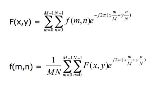
where f(m,n) is the pixel at coordinates (m,n), F(x,y) is the value of the image in the frequency domain corresponding to the coordinates x and y, and M and N are the dimensions of the image.

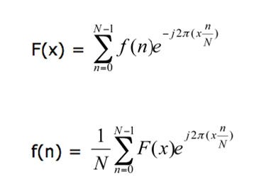
As the equations show, a naive implementation of this algorithm is very expensive. But the beauty of FFT is that it is separable; namely, the 2D transform can be split into two 1D transforms-one in the horizontal direction and the other in the vertical direction. The equation below shows the 1D transform in the horizontal direction.² The end result is equivalent to performing the 2D transform in the frequency space.

The FFT that is implemented in the application here requires that the dimensions of the image be a power of two. Another interesting property of FFT is that the transform of N points can be rewritten as the sum of two N/2 transforms (divide and conquer).³ This is important because some of the computations can be reused, which eliminates expensive operations.

The output of the Fourier transform is a complex number and has a much greater range than the image in the spatial domain. Therefore to accurately represent these values, they are stored as fl oats. Furthermore, the dynamic range of the Fourier coefficients are too large to be displayed on the screen, and hence these values are scaled [usually by dividing by the (Width × Height) of the image] to bring them within the range of values that can be displayed.⁴

The next section describes the implementation details of the FFT algorithm and its inverse in a GPGPU application.

---

² Sumanaweera, Thilaka, and Donald Liu, "Medical Image Reconstruction with the FFT." Chapter 48 in GPU Gems 2: Programming Techniques for High-Performance Graphics and General-Purpose Computation, Matt Pharr, ed., Addison Wesley, 2005.

³ Cooley, J. W., and Tukey, O. W., "An Algorithm for the Machine Calculation of Complex Fourier Series." Math. Comput. 19 (1965): 297-301.

⁴ Mitchell, Jason L., Marwan Y. Ansari, and Evan Hart, "Advanced Image Processing with DirectX® 9 Pixel Shaders." Section 4 in ShaderX2: Shader Programming Tips and Tricks with DirectX 9, Wolfgang F. Engel, ed., Plano, TX: Wordware Publishing, 2003. 

Implementation Details

Because the FFT is a divide-and-conquer algorithm, the various steps can be implemented in multiple passes in a shader by rendering the result of each pass to a texture. These steps are called butterflies, because of the shape of the data-flow diagram.

The FFT algorithm recursively breaks down a DFT of composite size N = n1n2 into n1 smaller transforms of size n2.

These smaller DFTs are then combined with size n1 butterflies, which themselves are DFTs of size n1 (performed n2 times on corresponding outputs of the sub-transforms) pre-multiplied by roots of unity (known as twiddle factors).⁵

The application employs four 2D textures: two for the ping-pong operations, one for the source data (for each pass), and one for holding the indices and weights for performing the butterfly steps.

The textures used for ping-ponging are marked as either a RenderTarget texture or a source depending on whether they are used as destinations or sources in the current pass.

This enables the shader to use the output of the previous pass as input for the current pass. Here are the steps to implement the FFT algorithm.

1. Compute the indices and weights for performing the butterfly operations.

2. Compute the log2(Width) horizontal butterflies.

3. Compute the log2(Height) vertical butterflies.

If the height and width of the image are equal, only one texture can be used for the butterfly values, for both the horizontal and vertical passes. Also note that in the vertical butterfly pass the input is the result of the horizontal butterfly pass.

In each butterfly pass the current pixel is combined with another pixel using a complex multiply and add operation and written to the current location. In other words if the current pixel is a, then

a = a + wb

where w is a complex number representing the weight and b is some other pixel. Each texel of the butterfly texture contains the locations of a, b and the value of w and passed to the shader by the application.

Note that for simplicity, only gray scale images are considered in the current implementation. However, extending the algorithm to multiple color channels is straightforward and only requires more textures for additional channels.

---

⁵ http://en.wikipedia.org/wiki/Butterfly_(FFT_algorithm)

Here is the shader program that computes the butterflies in the horizontal direction.

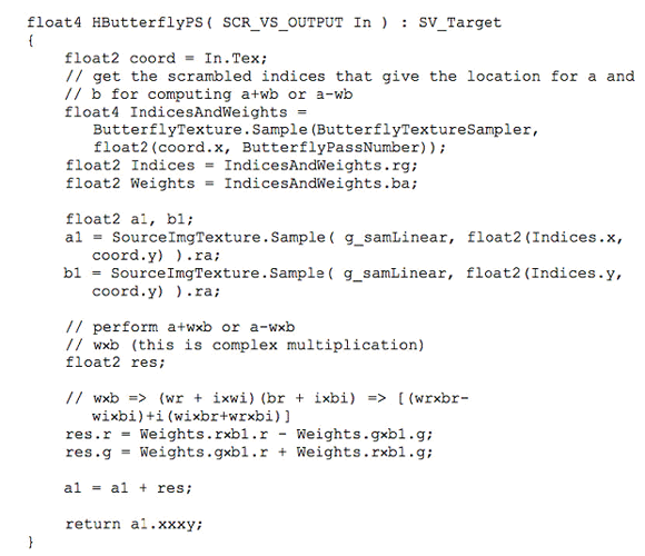
The shader looks up the butterfly texture for the indices of the two pixels to be combined and the weight. It then computes the result by performing the complex math a+wb or a-wb. To make matters simple, the sign is encoded as part of the weight and hence only the addition is performed in the shader program every time. The result is returned with the real value in the first three components and the imaginary value in the fourth component.⁶

To transform the image from the frequency domain to the spatial domain the exact same operations are performed but on the frequencies. Because the frequencies are not in the range to be displayed on the screen they are scaled by a factor of 1/(Width × Height) as shown.

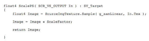
where ScaleFactor is set by the application to 1/(Width × Height). Finally the result is displayed in the normal mode by concentrating the lowest frequencies toward the center.⁷ Figures 1 and 2 show a gray scale image and the resulting image after applying FFT.

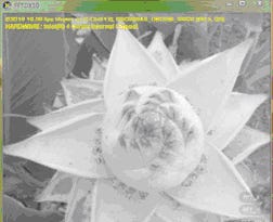
Figure 1. The original image displayed in gray scale.

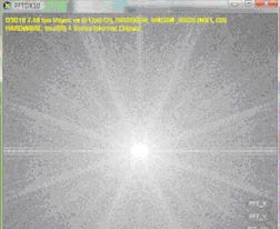
Figure 2. The normal mode of the image after applying the FFT.

Conclusion

This DirectX 10 application not only implements the FFT and its inverse but also serves as a framework for implementing image-processing algorithms. A CTexture class is implemented for handling 1D and 2D texture operations. The CTexture class supports various texture formats and can be easily extended to support 3D textures. Future work will focus on making the framework a plug-in architecture allowing developers to write image processing filters and plug their algorithms into the framework.

This article detailed the implementation of FFT and its inverse for transforming a 2D image from the spatial domain to the frequency domain and back. The advantage of representing an image in the frequency space is that performing some operations on the frequencies is much more efficient than doing the same in the image space. Many of the convolutions are just multiplications in the frequency domain (the computational cost in the image space is O(N2) versus O(Nlog(N)) in the Fourier space for N points). This enables efficient implementations of very large convolutions in image processing and other algorithms in many fields.

---

⁶ Mitchell, Jason L., Marwan Y. Ansari, and Evan Hart, "Advanced Image Processing with DirectX® 9 Pixel Shaders." Section 4 in ShaderX2: Shader Programming Tips and Tricks with DirectX 9, Wolfgang F. Engel, ed., Plano, TX: Wordware Publishing, 2003.  

⁷ Mitchell, Jason L., Marwan Y. Ansari, and Evan Hart, "Advanced Image Processing with DirectX® 9 Pixel Shaders." Section 4 in ShaderX2: Shader Programming Tips and Tricks with DirectX 9, Wolfgang F. Engel, ed., Plano, TX: Wordware Publishing, 2003.