[In this technical article originally printed in Game Developer magazine, Neversoft co-founder Mick West looks at how to efficiently implement fluid effects - from smoke to water and beyond - in video games, with example code.]

Fluid effects, such as rising smoke and turbulent water flow, are everywhere in nature but are seldom implemented convincingly in computer games. The simulation of fluids (which covers both liquids and gases) is computationally very expensive.

It's also mentally expensive, with even introductory papers on the subject relying on the reader to have math skills at least at the undergraduate calculus level.

In this two-part article, I will attempt to address both these problems from the perspective of a game programmer who's not necessarily conversant with vector calculus. I'll explain how certain fluid effects work without using advanced equations and without too much new terminology.

I'll also describe one way of implementing the simulation of fluids in an efficient manner without the expensive iterative diffusion and projection steps found in other implementations.

A working demonstration in ZIP form with source code accompanies this article; example output from this can be seen in Figure 1.

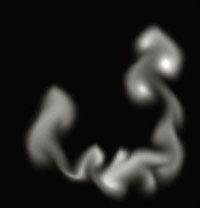
FIGURE 1 Smoke output is shown from the accompanying code.

Grids and Particles

There are several ways of simulating the motion of fluids, but they all generally divide into two common styles: grid methods and particle methods. In a grid method, the fluid is represented by dividing up the space a fluid might occupy into individual cells and storing how much of the fluid is in each cell.

In a particle method, the fluid is modeled as a large number of particles that move around and react to collisions with the environment, interacting with nearby particles. Let's focus first on simulating fluids with grids.

The simplest way to discuss the grid method is in respect to a regular two-dimensional grid, although the techniques apply equally well in three dimensions. At the most basic level, to simulate fluid in the space covered by a grid you need two grids: one to store the density of liquid or gas at each point and another to store the velocity of the fluid.

Figure 2 shows a representation of this, with each point having a velocity vector and containing a density value (not shown). The actual implementation of these grids in C/C++ is most efficiently done as one-dimensional arrays. The amount of fluid in each cell is represented as a float.

The velocity grid (also referred to as a velocity field, or vector field) could be represented as an array of 2D vectors, but for coding simplicity it's best represented as two separate arrays of floats, one for X and one for Y.

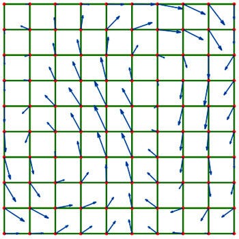
FIGURE 2 The fluid density moves over a field of velocities, with a density stored at each point.

In addition to these two grids, we can have any number of other matching grids that store various attributes. Again, each will be stored as a matching array of floats, which can store factors such as the temperature of the fluid at each point or the color of the fluid (whereby you can mix multiple fluids together).

You can also store more esoteric quantities such as humidity, for example, if you were simulating steam or cloud formation.

Advection

The fundamental operation in grid-based fluid dynamics is advection. Advection is basically the moving of things on the grid, but more specifically, it's moving the quantities stored in one array by the movement vectors stored in the velocity arrays.

It's quite simple to understand what's happening if you think of each point on the grid as an individual particle, with some attribute (density) and a velocity. Then you are familiar with the process of moving a particle by adding the velocity vector to the position vector. On the grid, however, the possible positions are fixed, so all we can do is move (advect) the quantity (density) from one grid point to another.

In addition to advecting the density value, we also need to advect all the other quantities associated with the point. This would include additional attributes such as temperature and color, but also the velocity of the point itself. The process of moving a velocity field over itself is referred to as self-advection.

The grid does not represent a series of discrete quantities, density or otherwise; it actually represents (inaccurately) a smooth surface, with the grid points just being sample points on that surface.

Think of the points as being X,Y vertices of a 3D mesh, with the density field being the Z height. Thus, you can pick any X and Y position on the mesh, and find the Z value at that point by interpolating between the closest four points. Similarly while advecting a value across the grid, the destination point will not fall directly on a grid point, and you'll have to interpolate the value into the four grid points closest to the target position.

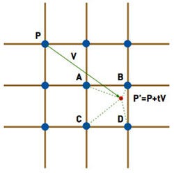
FIGURE 3 Forward advection: The value in P moves forward to A, B, C, and D. This dissipates it when moving diagonally.

In Figure 3, point P has a velocity V, which, after a time step of t, will put it in position P´=P+t*V. This point falls between the points A, B, C, and D, and so a bit of P has to go into each of them. Generally, t*V will be significantly smaller than the width of a cell, so one of the points A, B, C, or D will be P itself. There are various inaccuracies when advecting an entire grid like this, particularly that quantities dissipate when moving in a direction that is not axis-aligned. But this inaccuracy can be turned to our advantage.

Stam's Advection

Programmers looking into grid-based fluid dynamics for the first time will most often come across the work of Jos Stam and Ron Fedkiw, particularly Stam's paper "Real-Time Fluid Dynamics for Games," which he presented at the 2003 Game Developers Conference. He describes a very short procedure for making a grid-based fluid simulator.

In particular, he shows how to implement the advection step using what he calls a "linear backtrace," which simply means that instead of moving the point forward in space, he inverts the velocity and finds the source point in the opposite direction, essentially back in time. He then takes the interpolated density value from that source (which, again, will lay between four actual grid points), and moves the value into the point P. See Figure 4 for an example.

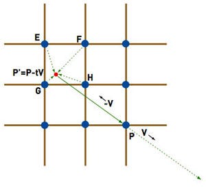
FIGURE 4 Reverse advection: The new value in P is gathered from E, F, G, and H, one of which (H) is usually the same point as P.

Stam's approach produces visually pleasing results, yet suffers from a number of problems. First, the specific collection of techniques discussed may be covered by an existing patent (U.S. #6,266,071), although as Stam notes, backtracing dates back to 1952. Check with a lawyer if this is a concern to you.

On a more practical note, the advection alone as Stam describes it simply does not work accurately unless the velocity field is smooth in a way termed mass conserving, or incompressible.

Consider the case of a vector field in which all the velocities are zero except for one. The velocity cannot move (advect) forward through the field, since there's nothing ahead of it to "pull" it forward. Instead, the velocity simply bleeds backward. The resultant velocity field will terminate at the original point, and any quantities moving through this field will end up there.

We can solve this particular problem by adding a step to the algorithm termed projection. Projection essentially smooths out the velocity by making it incompressible, allowing the backtracing advection to work perfectly and making the paths formed by the velocity "swirly," as if it were real water. The problem with this approach is that projection is quite expensive, requiring 20 iterations over the velocity field in order to "relax" it to a usable state.

Another performance problem with Stam's approach is that he uses a diffusion step, which also involves 20 iterations over a field. It's necessary to allow the gas to spread out from areas of high density to areas of low density. If the diffusion step were missing, solid blocks of the fluid would remain solid as they moved over the velocity field. Diffusion is an important cosmetic step.

Accounting Advection

If a velocity field is not mass conserving, then some points will have multiple velocity vectors from other points pointing toward them. If we simply move our scalar quantities (like density) along these vectors, there will be multiple quantities going to (or coming from) the same point, and the result will be a net loss or gain of the scalar quantity. So, the total amount of something such as the density would either fade to zero or gradually (or perhaps explosively) increase.

The usual solution to this problem is to make sure the vector field is incompressible and mass conserving. But as mentioned before, it's computationally expensive to implement. One partial solution is to make the advection step mass conserving, regardless of whether the velocity field is actually mass conserving. The basis of this solution is to always account for any movement of a quantity by subtracting in one place what is added in another.

Advection uses a source and destination buffer to keep it independent of update order. In Stam's implementation, the destination buffer is simply filled one cell at a time by combining a value from four cells in the source buffer and placing this value into the destination buffer.

To properly account for compressible motion, we need to change this copying to accumulating, and initially make the destination buffer a copy of the source buffer. As we move quantities from one place to another, we can subtract them in the source and add them in the destination.

With the forward advection in Figure 3, we're moving a quantity from point P to points A, B, C, and D. To account for this, we simply subtract the original source value in P from the destination value in P, and then add it (interpolated appropriately) to A, B, C, and D. The net change on the destination buffer is zero.

With the reverse advection in Figure 4, as used by Stam, the solution would initially seem to be symmetrically the same: Subtract the interpolated source values in E, F, G, and H from the destination buffer, and add them to P.

While this method works fine for signed quantities such as velocity, the problem here is that quantities such as density are positive values. They cannot drop below zero, as you cannot have a negative quantity of liquid.

Suppose that point E was one source point for two destinations P1 and P2, both of which wanted 0.8 of E. If we follow our initial plan and subtract 0.8*E from E and add 0.8*E to both P1 and P2, the net effect is zero, but now the value at E is negative. If we clamp E to zero, then there is a net gain of 0.6*E. If we subtract 0.8*E from the source value of E after updating P1, then when we update P2, it will only get 0.8*0.2*E, when clearly both P1 and P2 should get equal amounts. Intuitively, it seems they should both get 0.5*E, and the resulting value in E should be zero, leading to a net zero change.

To achieve this result, we create a list that for each point, noting the four points of origin for each and the fraction of each point they want. Simultaneously, we can accumulate the fractions asked of each source point. In an ideal world, this would add up to one, as the entire value is being moved somewhere (including partially back to where it started).

But with our compressible field, the amount of the value in each point that is being moved could be greater than or less than one. If the total fraction required is greater than one, then we can simply scale all the requested fraction by this value, and the total will be one. If less than one, the requesting points can have the full amount requested. We should not scale in this case, as it will lead to significant errors.

With the mass conservation of advection fully accounted for in both directions, it turns out that neither forward nor backward linear advection alone will produce smooth results. After some experimentation, I determined that applying forward advection followed by backward advection worked very well and gives a smooth and artifact-free flow of fluid over a compressible velocity field.

Now What?

We can now perform both forward and reverse advection in a mass-conserving manner, meaning we can move fluid around its own velocity field. But even though our velocity field does not need to be mass-conserving, we actually still want it to be, since the velocity fields of real world fluids generally are incompressible.

Stam solves this problem by expensively forcing the field to be fully mass conserving after every change. It's necessary, since the reverse advection requires it. The key difference is that since our advection step does not require the field to be mass-conserving, we're really only doing it for cosmetic purposes.

To that end, any method that rapidly approaches that state over several time steps will suit our purpose. That method, and the method of diffusion, can be found in the accompanying code, and I will discuss how they work in the next instalment of the article.

[EDITOR'S NOTE: This article was independently written and commissioned by Gamasutra's editors, since it was deemed of value to the community. Its publishing has been made possible by Intel, as a platform and vendor-agnostic part of Intel's Visual Computing microsite.]