[In this technical article, veteran coder Jovanovic looks at dynamic game-related effects like heat distribution models, explaining useful mathematical formulas that should help decrease the amount of programming.]

In games today, more and more realistic effects are expected, and the best way to get them is by using the correct physical models. The problem many of these models share is that they are represented with partial differential equations (PDE).

The solving of this type of equation is often avoided by using different types of tricks. It is sad to say, but in the end tricks are just tricks, and they don't give the correct solution - just something that looks like it.

There are two main reasons for using tricks. The first one is that they are usually much faster - but with the increase of CPU power we can give up some of the speed to get more reality. The second reason is that most people think solving PDEs is very complicated, and in many cases this simply isn't true.

In this article we'll show a standard method of solving PDEs and how to implement it. This method is called Finite Difference Scheme (FDS). It is not the most exact and stable method that exists, but is much better than using tricks, and it is the easiest to understand and implement.

A game example of the use of PDE

Let us try to show the advantages of using a mathematical model with PDE and the FDS method in a game. Let's say we wish to have a trampoline, or something like a rubber sheet that represents a wall that moves with the wind. How would it be implemented in a game? The approach in games today is to use a spring system.

Anyone who programmed spring systems knows this isn't the simplest task in the world. We have to create classes for nodes, springs, the hole system; and than calculate the forces from all the springs, and than apply the sum of forces corresponding to each node. And after all that work we get something that can often become numerically unstable.

Spring systems are actually great and very complex objects can be modeled with them, but in this case we don't need them. There is a much easier way.

The behavior of a trampoline, or the vibrating membrane, is one of the standard physical problems and one of the basic PDE. The equation that represents it looks something like this:

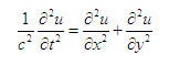
When someone sees something like this the natural reaction is "I'll stick with spring systems, since it's surely much easier." This is wrong for a couple reasons.

First, the implementation will be simpler; less programming will be needed. Second, the final result will look better because we used a better mathematical model, or in other words we modeled a trampoline and not just a bunch of nodes connected with springs. Third, there will be less calculation which means the code will work faster.

Heat Equation

While the trampoline is a good example for showing the power of using PDE, it is too complicated for the first contact with the implementation of this type of equation with FDS method.

Learning new methods is best with a simple example, and one of the simplest PDE is the Heat Equation, it models the problem of heat distribution. We shall solve it in one dimension, and in that case the equation looks like this:

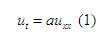
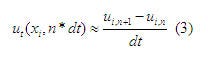
Here u(x,t) represents the heat distribution or what temperature is at each point of space at different moments in time. What do we wish to see in real time games? How things change over time. That is just what this equation shows us, the change. u_t is called the partial differential of u over t, and it represents how u changes over time (t). It is equal to:

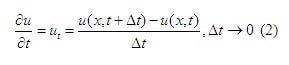
Since we are interested in viewing the heat distribution, we should first find a representation of u , in some useful way. Let's say that u_n(x) = u(x,dt*n) , where dt is our time step and n is some fixed number (it is not the same as t which is a variable).

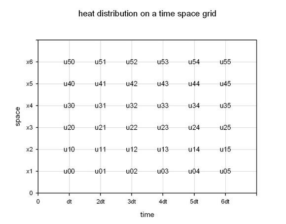
This way n*dt just represents some moment in time. Now we want to observe how the heat is distributed in space at that moment. The best way to do this is to use of a grid, x_i = x₀+i*h , where h is the step in the grid.

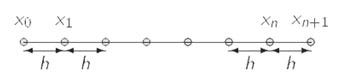
The heat distribution at moment n can be seen as an array of points u_in = u_n(x_i) . This is best understood by looking at this image:

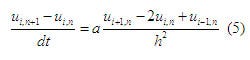
Now we get to the Finite Difference Scheme. The idea is to approximate u_t at each point in the grid. Using the time step dt we have the following approximation for equation (2):

This is actually a good approximation if dt is small. The next thing that we notice in the equation is u_xx . This is called the second partial derivative of u over x .

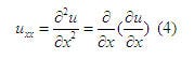
This is nothing more that doing the partial derivative twice on u over x . The partial derivative of u over x , represents how u changes over space( x ). The approximation will be exactly that.

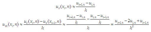
Now we can write the approximated version of equation (1) at every point in the grid.

We are at a point from where we can take a time step, or to move from a moment n at which we know how u looks, to moment n + 1 where we don't know how u looks. If we look closely at the equation (5) we notice that there is only one element that is at the time step n + 1 . So let us solve it:

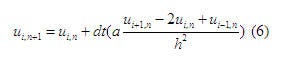
Equation (6) is the end of the simple use of FDS. Now we can add a mathematical "trick" to make it more precise. First let us take a look at equation (6), it is actually very similar to the approximation of the Euler method.

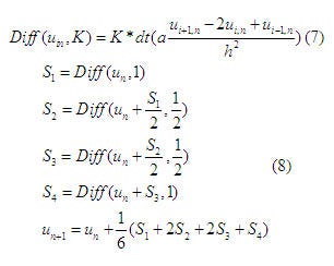
So we can use an approximation of Runge-Kutta (another time step method) instead to make it more accurate. It is calculated by the following formulas:

Adaptive grid

A big problem with FDS is that many times there is much more calculation than we actually need. It is easer to understand this if we imagine that we are heating a long metal wire in the middle. It will be very hot there and the heat will slowly move to the ends.

The heat distribution near the fire will be changing quickly, while it will be almost constant at the ends. It is obvious that we need more precise calculations near the fire than at the ends.

This is a situation that is quite common in many problems that we simulate with PDEs. Because of this characteristic, the idea of adding an adaptive grid (using different h at different parts of the problem space) to FDS appeared quickly.

This is when it starts to show its real power - due to the large increase in the speed of calculation. There are many articles written about this subject, but most of them are dedicated to mathematical aspects.

The implementation of this kind of grid in a computer program can turnout to be a much bigger problem than expected. When using an adaptive grid there are two important steps that need to be done.

The first is to create a grid that has high resolution at the correct places and that allows easy transition between indexes of high and low resolution areas. The second is to correct the corresponding equations. One method of solving these problems is explained in detail in this article.

Implementation

With the math out of the way, we can say a couple things about the software implementation. We shall explain it with some pseudo code, and some comments. As expected u will be kept in an array, but we will also need one more to keep a copy of it in the previous step.

double u[MAX], uprev[MAX]

Now we wish to translate equations (7,8) into some code. We will create a function to calculate Diff first, for all the elements in the array.

void Diff(double u[],double diff[],double K)
{
diff [0] = diff [MAX-1]=0;
for(int i =1; i< MAX -1;i++)
diff [i]= K*dt*a*( u[i+1] - 2*u[i] + u[i])/(h*h)


}

At this point we can say that a is a parameter that holds some physical characteristics and it can be set to 1. Notice that the first and the last elements in the array are set to 0. This is the border and things are a bit different there. Some explanations will follow in a bit. Using Diff we implement the approximation of Runge-Kutta:

void Calculate (double u[],double uPrev[])
{
double S1[Max], S2[Max], S3[Max], S4[Max];
doubleuTemp[Max],

uTemp = uPrev;
FixBorder(uTemp);
Diff(uTemp, S1, 1);

uTemp = uPrev + 0.5*S1;
FixBorder(uTemp);
Diff(uTemp, S2, 0.5);

uTemp = uPrev + 0.5*S2;
FixBorder(uTemp);
Diff(uTemp, S3, 0.5);

uTemp = uPrev + 1*S3;
FixBorder(uTemp);
Diff(uTemp, S4, 1);

u = uprev + (S1 + 2*S2 + 2*S3 + S4)/6;
FixBorder(u);

}

This function looks pretty much as expected, besides FixBorder appearing out of the blue. This is one more problem with FDS - the border. It is obvious that the array has to have some beginning and some end, but at these points we can't calculate Diff. How we solve this problem is very important, because in a number of time steps this will affect all the elements in the array.

Actually what we do at the border can have many different effects on our function which corresponds to different physical models. A lot of research has been done in math about this subject and many different approaches have been used. In our example we shall use a simple one, that isn't very mathematically strict. We shall just keep "going in the same direction".

void FixBorder(double u[])
{
u[0] = u[1] + (u[1]-u[2]);
u[Max-1] = u[Max-2] + (u[Max-2]-u[Max-3]);
}

Finally we have the calculation loop.

Init(u);
while(simulation)
{
uprev = u;
CalculatorFDSHeat->Calculate(u,uprev)
}

The use of the scheme has been put in a class, with which we wish to signify that the use of FDS is practically the same for all possible problems. The only difference would be Diff that is used in the implementation of Runge-Kutha time step.

If an adaptive grid was used there would be some extra lines. First some that would create the grid before the main loop, and some that would recalculate the grid every m step.

Conclusion

There are many processes in nature that have been translated into PDEs, and with this method they could be added to games. This was a presentation of an improved FDS and its implementation, for a very simple problem.

The use of it for more complex problems would in its basics have the same steps. They are finding the correct equations for the problem, creating the scheme, creating the adaptive grid and implementing the functions.

As an example of a problem in 2+1 dimensions you can read this article. This is a powerful method, but solving PDEs is a very hard problem in many cases, and this method might not always give very accurate and stable results.

There are other methods like implicit FDS, finite elements, and the use of Fourier Transform that may be able to solve them, but in some cases it is still best just to use tricks.