Daily news, dev blogs, and stories from Game Developer straight to your inbox
Sponsored By
Practical Fluid Dynamics: Part 2
Following up his <a href="http://www.gamasutra.com/view/feature/1549/practical_fluid_dynamics_part_1.php">popular recent article</a>, Neversoft co-founder Mick West explains the technical details - including source code - of creating dynamic fluid systems such as smoke for video games.
12 Min Read

[Following up his popular recent article, Neversoft co-founder Mick West explains the technical details - including source code - of creating dynamic fluid systems such as smoke for video games.]
In the last article, I gave an overview of the nuts and bolts behind simple two-dimensional fluid dynamics using a grid system. This time, I explain how programmers can achieve a reasonable level of realism with fluid dynamics without too much expensive iteration.
I'll also continue with my goal of explaining how everything works by using nothing more complex than basic algebra.
To recap the last column: we have a velocity field, which is an array of cells, each of which stores the velocity at a particular point. Remember this is a continuous field, and we can get the velocity at any point on the field surface (or in the field volume for 3D), by interpolating between the nearest points on the field.
We also have a matching field of density. The density field represents how much of the fluid or gas is in a particular grid cell. Again, we're dealing with a continuous field, and you can get a density value for any point in the simulated space by interpolating.
I then described the process of advection, which is the moving of values in one field (for example, the density field), over the velocity field. I described both forward advection and reverse advection, where the quantities in the field are respectively pushed out of a cell or pulled into a cell by the velocity at that cell. The advection process worked well if you performed forward advection and then follow it with reverse advection.
Incompressible Fields
Reverse advection in particular only works if the velocity field is in a state termed incompressible. But what does that mean?
You may have heard that "water is incompressible," meaning you can't squeeze water into a smaller volume than it already occupies. Compare this with gasses such as air, which can clearly be compressed. Picture, for example, a diver's air tank. The tank contains a lot more air than the volume occupied by the tank. But if you were to take that tank and fill it with water, and then somehow push in another pint of water, the tank would explode.
Actually, water is in fact compressible, very slightly, since it's physically impossible to have a truly incompressible form of matter. The incompressibility of a material is measured by a metric called a "bulk modulus." Air's bulk modulus is about 142,000, whereas for water, it's 2,200,000,000 or approximately 15,000 times as much.
By comparison, the least compressible substance known to humankind, aggregated diamond nanorods, are just 500 times more incompressible than water. So for most practical purposes, you can imagine water as being incompressible.
Because water is considered incompressible, there cannot be more water in one cell than in another when considering a solid volume of water. If we start out with an equal amount of water in each cell, then after moving the water along the velocity field (advecting), we can't increase or decrease the amount of water in each cell. If this happens, then the velocity field is incompressible or mass conserving.
Pressure
You can think of the pressure at a particular node as being the difference in density between a cell and its neighbors. The pressure of water will be the same throughout the density field since it's incompressible. If we think of a node as having a series of inputs and outputs during the advection process, then in an incompressible field, the sum of input is equal to the sum of outputs (see Figure 1A). When we move the water along its incompressible velocity field, the density at each node remains constant, and hence the pressure remains constant.
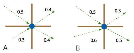
On the other hand, if the velocity field happens to be structured in such a way that for some cells more is going into them than is coming out, the velocity field is compressible (see Figure 1B). When the density of the fluid is advected across a compressible velocity field, the density in individual cells will increase or decrease.
If we simply keep advecting the density, all the matter will eventually be compressed into the cells of the velocity field that have a net gain of input over output. If we were not performing accounting in our advection step (as explained last month), then there would be a net loss in density (the field is not mass conserving).
Let's step back from our abstraction for a second and consider what prevents this situation from happening in real life. If more of a fluid flows into a cell than flows out, then the density of that cell increases relative to its neighbors, and hence the pressure in that cell increases.
High pressure in a cell creates an acceleration force on the neighboring cells, increasing their velocity away from that cell, thereby increasing the outflow rate from the cell and evening out the imbalance. As with the atmosphere, fluid flows from an area of high pressure to an area of low pressure.
Applying Pressure
Listing 1: Pressure Differential
for (int x = 0; x < m_w-1; x++) {
for (int y = 0; y < m_h-1; y++) {
int cell = Cell(x,y);
float force_x = mp_p0[cell] - mp_p0[cell+1];
float force_y = mp_p0[cell] - mp_p0[cell+m_w];
mp_xv1[cell] += a * force_x;
mp_xv1[cell+1] += a * force_x;
mp_yv1[cell] += a * force_y;
mp_yv1[cell+m_w] += a * force_y;
}
The pressure differential between two cells creates an identical force on both cells.
Listing 1 shows the code for applying pressure. Here mp_p0 is the array that stores the density (which is equivalent to the pressure, so I actually refer to it as pressure in the code). The arrays mp_xv1 and mp_yv1 store the x and y components of the velocity field. The function Cell(x,y) returns a cell index for a given set of x and y coordinates. The loop simply iterates over all horizontal and vertical pairs of cells, finds the difference in pressure, scales it by a constant (also scaled by time), and adds it to both cells.
The logic here is slightly unintuitive, since physics programmers are used to the Newtonian principle that every action has an equal and opposite reaction-yet here when we add a force, there's no opposing force, and we don't subtract a force from anywhere else.
The reason is clear if you consider what's actually happening. We're not dealing with Newtonian mechanics. The force comes from the kinetic energy of the molecules of the fluid, which are randomly traveling in all directions (assuming the fluid is above absolute zero), and the change to the velocity field actually happens evenly across the gradient between the two points. In effect, we're applying the resultant force from a pressure gradient to the area it covers (which is two cells here), and we divide it between them.
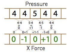 Here's an example: Just looking in the x direction, we have a flat pressure field, with one cell denser that the rest. The cell densities are 4, 4, 5, 4, 4. The gradients between the four pairs of cells is 0, -1, 1, and 0 Adding this to each cell (ignoring scaling), we get: 0, -1, 0, 1, and 0 (see Figure 2).
The cells on either side of the high-pressure cell end up with a velocity pointing away from that cell. Consider now what will happen with the advection step. The reverse advection combined with forward advection will move the high-pressure cell outward, reducing the pressure and force. The fluid moves from an area of high pressure to low pressure.
Effectively, this makes the velocity field tend toward being incompressible and mass conserving. If there's a region that's increasing in density, then the resultant increase in pressure will turn the velocity field away from that area, decreasing the density in that area. Eventually, the velocity field will either become mass conserving (mass just circulating without density change) or it will stop (become zero). See Listing 1.
Ink And Smoke
What we're modeling here is motion within a fluid, such as air swirling around inside a room, and not the overall motion of a volume of water, such as water sloshing around in a cup. This method as it stands does not simulate the surface of the fluid. Visualizing the fluid itself is not very interesting, since a room full of air looks pretty much the same regardless of how the air moves.
What's more visually interesting is the situation in which some substance is suspended by that fluid, carried around by the fluid. With water, we might have silt, sand, ink, or bubbles. In air, we could see dust, steam, or smoke. You can even use the velocity field techniques outlined here to move larger object, like leaves or paper in a highly realistic manner.
It's important that what we're talking about is a suspension of one substance in another. We are generally not so interested in simulating two fluids that do not mix (like oil and water).
Games typically feature burning and exploding things, so smoke is a common graphical effect. Smoke is not a gas, but a suspension of tiny particles in the air. These tiny particles are carried around by the air, and they comprise a very small percent of the volume occupied by the air. So we do not need to be concerned about smoke displacing air.
In order to simulate smoke, we simply add another advected density field, where the value at each cell represents the density of smoke in that region. In the code, I refer to this as "ink." It's similar to the density of air, except the density of smoke or ink is more of a purely visual thing and does not affect the velocity field.
Heating Up
One final ingredient that often goes along with a fluid system like this one is the heat of the fluid or gas at each location. Sources of smoke are usually hot, which heats up the air the smoke initially occupies, causing the smoke to rise because higher temperatures mean more energy, which means the fluid molecules are moving faster, which means higher pressure, which means lower density (remember density is only proportional to pressure at constant temperature), which makes the hot air rise.
Now, that's a complex sequence of events, but it's initially simpler to just model the result "hot air rises" and have the relative temperature of a cell create a proportionate upward force on the velocity field at that cell. We can do this trivially by adding a scaled copy of the heat field to the Y velocity field.
Similarly, rather than attempt to model the effects of heat in the initial phases of a simulation, I found it easier to simply model the expected results. So, although a flame creates heat which makes the smoke rise, more pleasing results were found by "manually" giving the volume of air around the flame an initial upward velocity and letting the heat take it from there.
With more complex systems, such as an explosion, the fiddly physics happen in the first tenth of a second, so you can just skip over that and set up something that looks visually pleasing with our simplified physics.
Filtering Out Artifacts
The simplistic application of forces we perform for acceleration due to pressure (Figure 2) has the tendency to introduce artifacts into the system. These typically appear as unnatural looking ripples. The way to deal with them is to smooth out the velocity and pressure fields by applying a simple diffusion filter.
If you use the Stam-style reverse advection with projection, you have to use a computationally intensive filter, iterating several times. But with the inherent diffusion of forward advection, in cooperation with the accuracy of the combined forward and backward accounted advection, we can get away with a single iteration.
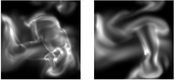
It's often difficult to see exactly what effect a change can have on a fluid system. The fluid is very complex looking, and small changes to parameters often have an outcome that's not immediately obvious. The ideal way to solve this problem is to set up your system so you can run two copies of the same system in parallel, with one using the modified parameters. The difference becomes obvious. Figure 3 shows such a comparison.
Fluid Ideas
I've glossed over a few other important aspects here, but details of these aspects can be found in the accompanying code.
Be sure to pay particular attention to how you handle the cells that are at the edge of the system, as the differing number of neighbors has a significant effect. At the edges of a system you have the option of reflecting, wrapping, or zeroing values, depending on what you want.
By wrapping in one direction, you essentially get a tiling animated texture in that direction, which could be used as a diffusion or displacement map for the surface of a moving stream of fluid.
There's also the issue of friction. Motion in a fluid is generally quite viscous, which can be implemented as a simple friction force that applies to the velocity field. If there's no friction in the fluid it will slosh around forever, which is generally not the desired effect. Different viscosity settings give very different visual results.
There is a large number of variables that you can tweak to give radically difference visual results, even in my rather simple implementation. Spend some time playing with these values just to see what happens.
[EDITOR'S NOTE: This article was independently published by Gamasutra's editors, since it was deemed of value to the community. Its publishing has been made possible by Intel, as a platform and vendor-agnostic part of Intel's Visual Computing microsite.]
Read more about:
FeaturesAbout the Author(s)
You May Also Like