Author: by John Van Drasek III

[Simulating convincing waves is mathematically complex and computationally taxing. In this sponsored article, part of the Intel Visual Computing microsite, John Van Drasek III, David Bookout and Adam Lake tackle the problem with DirectX 10.]

Abstract Summary

The simulation of ocean waves provides a significant challenge to computer graphics. Offline rendering yields phenomenal results, but the computational cost is high. The ability to generate waves in real time that resemble actual ocean waves is highly desirable. In this article we describe an implementation of a real-time shallow ocean wave simulation using Microsoft DirectX 10. Our simulation produces a variety of wave shapes and allows the designer to tune wave parameters in real time.

Introduction and Previous Work

Simulating ocean waves has been a challenging goal for both offline and real-time renderings. Early publications in the graphics literature date back to Peachey (1986) and Fournier (1986), but these publications refer to a number of wave simulations that were developed as early as 1981 and the film Carla's Island by Nelson Max (1981). For game developers, a continuing degree of realism has tracked the performance capabilities of hardware. These techniques can be partitioned into two categories: offline and real-time. In both of these categories, water simulation techniques are classified as those that simulate only the water surface and those that simulate the entire water volume.

Offline rendering lets us increase the physical accuracy without regard to the tight time constraints we have in real-time game engines. Many attempt to simulate the fluid mechanics using solutions of the Navier-Stokes (NS) equations. In computational fluid dynamics (CFD) an area or volume approximation is used to calculate an accurate solution to the NS equations (Wang 2007;Stam 1999; Foster 2001). Particle systems can also be used to create solutions to the NS equations. Examples include smoothed particle hydrodynamics (SPH) and level set methods1.

Real-time wave simulation also has two areas of research: treatment of the water as a 3D volume and treatment of the water as a 2D surface. Previous work using a volume-based approach includes that of Thürey (2007). Because of the reduced computational complexity of the surface simulations, the majority of work for game developers has been in this realm. The technique that treats the wave simulation as a surface was made popular by Tessendorf (2001), and relies on treatment of the surface in the Fourier domain. The corollary to the Tessendorf approach is known as the "sum of sines" (Isidoro 2002; Finch 2004; Lake, Van Drasek III, and Reagin 2005; Lake and Reagin 2005). Most recently, an interactive simulation that includes interaction with floating objects (Yuksel 2007) has been published. Although still simulating only the surface, Yuksel uses a particlebased approach.

Observations made by oceanographers and surf science authors provide data that reveals the behavior of ocean waves. Tessendorf refers to this method as a phenomenological approach. It produces results that work well to reduce the complexity in the simulation.

Our real-time parametric shallow wave simulation was written using DirectX 10 and provides a complete framework for future work on breaking-wave geometry simulations. The approach uses the work of Tessendorf, Finch, and Isidoro for the surface representation and the sum of sines method for generating wave shapes. Each vertex in the water surface mesh is calculated independently from other points in the mesh, which makes our wave simulation a good candidate for parallel workloads.

We begin by presenting the theory behind our wave simulation. Next we describe the approach used to create waves and manipulate their shape as they move into shallow water, and then we give the details of the normal mapping method used to simulate the surface effects. Finally, we provide performance numbers and discuss the results of this simulation.

Theory

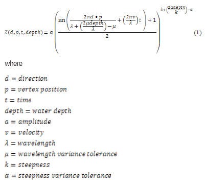
The fundamental component for our shallow wave simulation is the sine wave. A parameterized sine function allows control over the wavelength, amplitude, velocity, direction, and steepness of a wave for some point in the mesh at some time step. The inputs for the function are the direction, vertex position, time, amplitude, velocity, water depth, wavelength, wavelength variance tolerance, steepness, and steepness variance tolerance. The function returns a height value that is used to displace the z dimension of the water surface mesh. We summarize our approach, adopted from Finch.

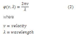
It is important for the phase of the wave to remain unchanged from one adjustment to the next. Maintaining a constant phase ensures smooth visual transitions when adjustments are made to the wave. Prior to changing the velocity and wavelength values, the phase is calculated. The inputs for the function that calculates the phase are velocity and wavelength. The output is the phase constant.

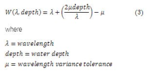
As a wave enters shallow water, the wavelength and velocity decreases while the steepness increases. The wavelength will begin to shorten when the depth of the water is less than one half of the wavelength. The inputs for the function that adjusts the wavelength are wavelength and water depth. The output is the adjusted wavelength.

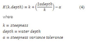
The steepness of the wave is adjusted after the wavelength has been adjusted. In our simulation we chose to adjust the steepness at the same rate as the wavelength, resulting in the two functions looking very similar. The inputs for the function that adjusts the steepness are steepness and water depth. The output is the adjusted steepness.

Now that we have adjusted the height of the vertices in our mesh with the parameterized sine function in equation (1), we need to compute the surface normal to use in our lighting calculations. The surface normal at a given vertex is calculated using differentiation (Finch). Differentiating in the x and y directions gives the rate of change of the surface and becomes the normal at the vertex we are evaluating. These derivations are known as the binormal and the tangent vectors, respectively. The binormal and tangent vectors create a matrix commonly referred to as a "tangent space matrix." The surface normal is multiplied by the tangent space matrix to properly orient it on the surface of the wave.

Implementation

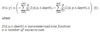
The calculations required for each vertex do not require any information from neighboring vertex locations or from previous iterations of the algorithm. The vertex shader is responsible for displacing vertex locations, calculating surface normals of the geometry, and applying the view transformations. The pixel shader is responsible for texture mapping, scrolling texture and normal maps across the surface, surface lighting effects, and setting transparency.

To displace the vertex locations in our shader, we will need initial wave parameters passed from the application code. To make it easier to pass the data between the different functions in the shader, we defined a structure that contains the parameters for our wave. First, we sample the height map to get the depth for the current vertex location, and then we loop through each of our waves. For each wave we get the trajectory from the dot product of the direction and position, and then we adjust the wavelength and the steepness based on the water depth. Using our adjusted wave parameters, a new position value is returned from the sine function for each wave in our simulation. We use each of these new position values, summing them, to displace the vertex in the z dimension on our water surface mesh.

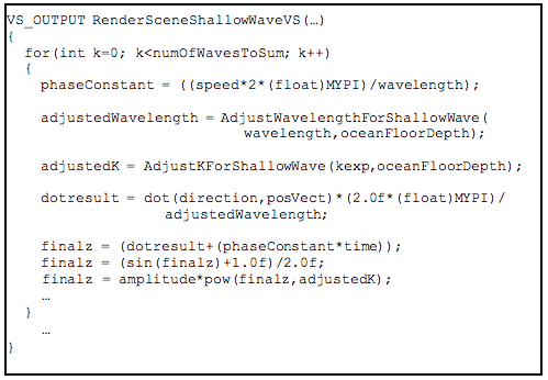
Code Listing 1. Vertex shader code associated with equation (1) showing the result of the sine function and its parameters used to adjust the z dimension of the water surface mesh.

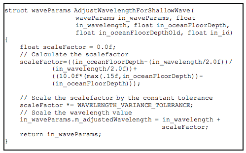
Code Listing 2. Vertex shader function that adjusts the wavelength based on some water depth value. Part of this calculation is simulating the shoreline surge by rapidly expanding the wavelength at a certain depth.

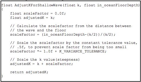
Code Listing 3. Vertex shader function that adjusts the steepness of the wave.

The Ocean Floor Representation

Chosen for artist control, our shallow wave simulation uses a height map to represent the ocean floor. The height map is a grayscale image, in which black represents the deepest value of 1 and white represents the shallowest value of 0. This height map has two functions: (1) displace the vertices of the ocean floor to show the depth of the water, and (2) provide a lookup table for values in which the wave can be adjusted.

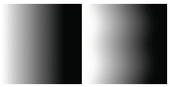
Figure 1. Two different sample height maps used for the ocean floor.

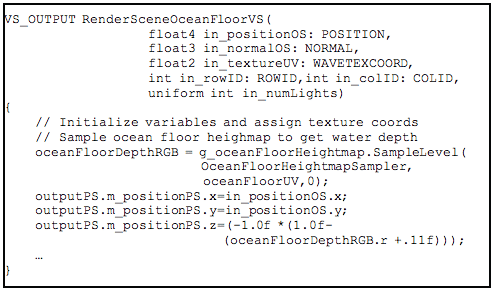
Code Listing 4. Vertex shader function to adjust the vertices on the ocean floor.

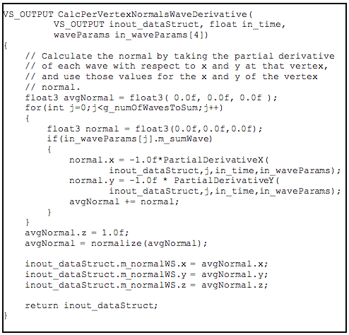
Code Listing 5. Vertex shader function to calculate the surface normal of the geometry by taking partial derivatives.

Surface Effects

The pixel shader begins by using the application-defined wind direction and wind speed variables to control the textures and normal maps that scroll across the surface. Then for each light in the scene a specular component is added to the lighting equation. The specular combined with the transparency of each texture layer helps to create a shimmering effect on the water surface.

The following sections describe each equation in the simulation along with short code segments to demonstrate the High Level Shader Language HLSL implementation.

We used normal mapping to simulate the ocean surface effects- high frequency surface waves and shimmering light effects. This approach helps to give the surfaces some depth without moving vertices. The calculation is done per pixel and is only a modification to the surface normal used in the lighting equation.

The use of layered textures allows the simulation of surface water effects. Texture maps and normal maps scroll across the mesh to simulate these effects. This allows a different combination of normals to be used in the lighting calculations, at each pixel, for every iteration of the simulation.

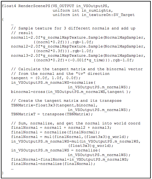
Code Listing 6. Pixel shader code to calculate the surface normal from the normal maps that scroll across the surface of the water.

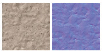
Figure 2. The texture and normal map used for the ocean floor.

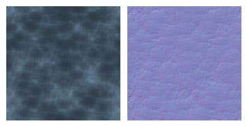
Figure 3. The texture and normal map used for the ocean surface.

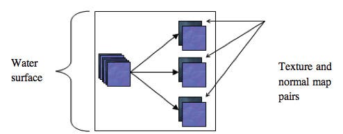
Figure 4. The texture map and normal map pairs scroll across the surface in different directions.

Performance

Our implementation of shallow waves runs in real time on a NVIDIA GeForce 8800 GTX 768 MB graphics card. To determine the performance of this algorithm we measured the number of frames per second (FPS) for varying mesh dimensions. The results in Figure 6 show the FPS obtained from the different mesh dimensions used.

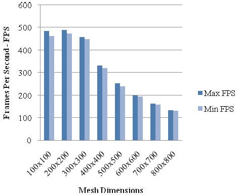
Figure 5. The graph shows the frame rates for varying mesh dimensions used in the shallow wave simulation.

Results

Our parametric shallow wave implementation is a flexible tool that can be used to develop ocean scenes for games. The simulation is fully parameterized allowing the designer to view the resulting wave shapes immediately after making adjustments. Because the simulation runs in real time and makes use of the DirectX 10 API, it is a desirable framework to use in real-time breaking-wave research.

To create our waves, we use the initial wave parameters and a height map to look up the water depth at each grid location. This approach results in an algorithm that is highly parallelized because we do not rely on data from neighboring grid locations or stored from previous iterations of the algorithm.

Results

Conclusion

Our parametric shallow wave simulation is a flexible tool and was written with the DirectX 10 graphics API. The simulation gives game designers a way to create and modify various shallow water wave shapes in real time.

When rendering in real time, it is difficult to achieve similar results to offline rendering because of the time constraints imposed by consumer graphics hardware.

Simplifications to equations must be made to reduce the computational cost in order to conform to the tight time restrictions.

Future Work

One interest for future work is the real-time simulation of breaking waves using phenomenological data acquired from scientific observation. Having a tool that could procedurally generate breaking waves for use in a real-time application has many benefits and remains an open challenge to computer graphics.

The interaction between the ocean water and the beach is also an interesting area for future work. Texturing for wet versus dry sand could be implemented at the point where the water surface touches the shoreline on the beach. Simulating wave spray and foam from breaking and crashing waves as well as when water rushes onto the beach would also be an interesting addition.

Our implementation assumes a monotonically sloping ocean floor or a flat ocean floor as shown in Figure 6. When the ocean floor is not monotonic (Figure 7), two different depth inputs to the same function produce two wave shapes in different locations on the water surface. That is, for a given w and t, the values d0 and d1 exist such that d0 != d1 and F(w,t,d0) = F(w,t,d1), The ability to handle non-monotonic slopes would allow more interesting features to be added to the ocean floor.

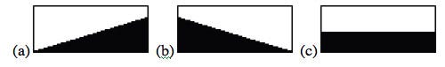
Figure 6. (a) A monotonically increasing ocean floor, (b) a monotonically decreasing ocean floor, and (c) a flat ocean floor.

Figure 7. An ocean floor that produces two wave shapes in different locations on the water surface.

Acknowledgements

We would like to thank Stephen Junkins, Jay Connelly, Gary Baldes, and Allen Hux for giving us the time and resources that allowed us to work on this exciting project.

References

Enright, Douglas, Stephen Marschner, and Ronald Fedkiw. 2002. Animation and Rendering of Complex Wave Surfaces. Proceedings of SIGGRAPH 2002, 736-744.

Finch, Mark. 2004. Effective Water Simulation from Physical Models. GPU Gems: Programming Techniques, Tips, and Tricks for Real-Time Graphics, Randima Fernando ed., 5-29.

Foster, Nick, and Ronald Fedkiw. 2001. Practical Animation of Liquids. Proceedings of ACM SIGGRAPH 2001, 23-30.

Fournier, Alan. 1986. A Simple Model of Ocean Waves. Proceedings of ACM SIGGRAPH 1986, 75-84.

Gomez, Miguel. Interactive Simulation of Water Surfaces. Game Programming Gems 1, Mark Deloura ed., 187-194.

Hinsing, Damien, Fabrice Heyret, and Marie-Paule Cani. 2002. Interactive Animation of Ocean Waves. Proceedings of ACM SIGGRAPH/Eurographics 2002 Symposium on Computer Animation, 161-166.

Isidoro, John, Alex Vlachos, and Chris Brennan. 2002. Rendering Ocean Water. Direct3D ShaderX: Vertex and Pixel Shader Tips and Tricks, Wolfgang Engel ed., 347-356.

Kim, Janghee, Deukhyun Cha, Byungjoon Chang, et. al. 2006. Practical Animation of Turbulent Splashing Water. Proceedings of ACM SIGGRAPH/Eurographics 2006 Symposium on Computer Animation, 335-345.

Lake, Adam, John Van Drasek III, and David Reagin. 2005. Real-Time Breaking Waves Poster, presented at GDC 2005.

Lake, Adam, and David Reagin. 2005. Real-Time Deep Ocean Simulation on Multi-threaded Architectures. Intel Web site, http://www. intel.com/cd/ids/developer/asmo-na/eng/200084.htm.

Longuet-Higgins. 1980. M. S. A Technique for Time-Dependent Free- Surface Flows. Proceedings of the Royal Society of London. Series A, Mathematical and Physical Sciences, 371, no. 1747 (Aug. 4, 1980): 441-451.

Parametric Solutions for Breaking Waves. 1982. J. Fluid Mechanics 121:403-424.

Losasso, Frank, Frédéric Gibou, Ron Fedkiw. Simulating Water and Smoke with an Octree Data Structure. ACM Trans. Grap. 23, (3): 457-462.

Nelson, Max. 1981. Carla's Island. Appeared in issue 5 of the SIGGRAPH Video Review, 1981.

Mead, Shaw. 2003. Keynote Address: Surfing Science. Proceedings of the 3rd International Surfing Reef Symposium, Raglan, New Zealand. (June 22-25, 2003): 1-36.

Mead, Shaw, and Kerry Black. Predicting the Breaking Intensity of Surfing Waves. Special issue of the Journal of Coastal Research on Surfing (in press), 103-130.

Mihalef, Viorel, Dimitris Metaxas, and Mark Sussman. 2004. Animation and Control of Breaking Waves. In ACM SIGGRAPH 2004 Symposium on Computer Animation, 315-323.

Miller, R. L. 1976. Role of Vortices in Surf Zone prediction: sedimentation, and wave forces. Beach and Nearshore sedimentation, Soc. of Economic Paleontologists and Mineralogists, Tulsa, Oklahoma, 92-114.

Peachey, D. R. 1986. Modeling Waves and Surf. Proceedings of SIGGRAPH 1986, 253-262.

Schneider, Jens, and Rudiger Westermann. 2001. Towards Real- Time Visual Simulation of Water Surfaces. Proceedings of the Vision Modeling and Visualization Conference 2001, Stuttgart, Germany, (Nov. 21-23).

Stam, Jos. 1999. Stable Fluids. Proceedings of SIGGRAPH 1999, 121-128.

Tessendorf, Jerry. 2001. Simulating Ocean Water. In Simulating Nature: Realistic and Interactive Techniques, ACM SIGGRAPH 2001 Course #47 Notes.

Thürey, N., F. Sadlo, S. Schirm, et. al. 2007. Real-time Simulations of Bubbles and Foam within a Shallow Water Framework. Proceedings of ACM SIGGRAPH/Eurographics 2007 Symposium on Computer Animation, 191-198.

Wang, Huamin, Gavin Miller, and Greg Turk. 2007. Solving General Shallow Wave Equations on Surfaces. Proceedings of ACM SIGGRAPH/ Eurographics 2007 Symposium on Computer Animation, 229-238.

Yuksel, Cem, Donald H. House, and John Keyser. 2007. Wave Particles. Proceedings of SIGGRAPH 2007, 99.

Index for Water Simulation. 2004. http://www.vterrain.org/Water/.