Author: by Marko Kylmamaa

Introduction

Creating a post-processing framework for your game engine is a powerful way to customize the look of your game and add a number of high-end features from basic blooming to color space manipulation and image perturbation.

Post-processing in itself is a relatively simple area of graphics programming, however there are some nuances which have to be paid attention to when using the 3D hardware to operate in 2D space.

The article will start by covering some basics for 2D programming with Direct3D and touching a bit on pixel alignment which is sometimes overlooked when implementing 2D features, and will then go further into optimization techniques for hardware and give basic ideas for certain special effects.

The Basics of Working in 2D

Work Buffers

The basic setup for a post-processing framework is to allocate one or more auxiliary buffers (other than the back-buffer) for rendering the scene, and then copy the rendered scene from this buffer to the back-buffer through a number of post-processing filters. A number of varying size auxiliary buffers may be needed for different special effects, for multiple pass filters or for example storing the previous frame’s data.

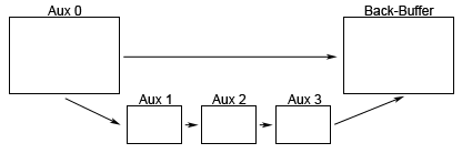
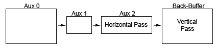
An example setup with 4 auxiliary work buffers and a back-buffer.

In the illustrated case the Aux 0 is used as the real render target throughout the scene, and smaller Aux 1-3 buffers are used during the post-processing as intermediary stages when transferring the scene through various filters to the back-buffer for displaying.

Addressing by Pixel

To address the source texture by pixel, the source texture coordinates have to be translated into pixels, which is done with the following formula:

dx = 1/TextureWidth
dy = 1/TextureHeight

This gives you dx,dy which are the pixel deltas in the UV space of 0-1.

Pixel Alignment

Special care must be taken in correctly mapping the source and target textures to the pixels centers for the hardware interpolation to yield the correct results. If the pixels are not perfectly aligned, the hardware may end up sampling in-between the intended pixels causing the output color to be an undesired blend of more than pixel. Also in the case of effects using a feed-back loop of the screen, a color bleeding may be produced.

In Direct3D, the texture coordinates originate at the top-left corner of the first texel, while the screen space coordinates originate at the center of the first pixel, as illustrated in the following figure.

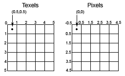
This means that when aligning the source texels to target pixels, the drawn target quad must originate from the screen coordinate (-0.5,-0.5), in pixels, in order for it to match with the top-left corner of the source texture (0,0).

Basic Setup

The basic setup for the post-processing framework would be as follows.

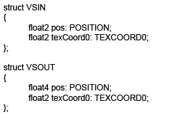
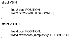
The HLSL code sample for vertex and pixel shader input
and output structures for a simple post-processing framework.

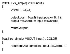
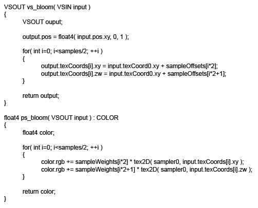
The HLSL code sample for basic vertex
and pixel shaders for the post-processing framework.

The code shown above doesn’t actually do anything except for passing the rendered scene from the auxiliary work buffer to the back-buffer. However it contains the fundamentals for adding on more complex post-processing effects.

Optimizations

Per-Vertex vs. Per-Pixel

For certain effects, per-pixel processing may be prohibitively expensive, and when running on lower-end hardware the pixel shader instruction sets may be too limited. In this case it is useful to break the rendered target quad into multiple smaller ones, so the heaviest computation can be moved either to the vertex shader or the CPU. This allows the results to be interpolated between the vertices, or the vertex coordinates to be modified for effects such as image perturbation.

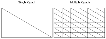
The image illustrates simple and highly tessellated target quads.

Using the Hardware Filtering

One way to make the most use of the hardware is to use the linear and bilinear hardware filtering to your advantage. Typically especially the lower end pixel shaders allow for a very few texture samples to be taken per-pixel. The number of sampled texels can be increased by enabling either linear or bilinear filtering of the source texture, and taking the source samples between the texels. This way the number of samples can be increased, for example, from 4 to up to 16 samples with very little additional cost.

This technique is illustrated in the following image:

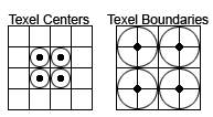
The black dots represent the sampling locations,
and the surrounding circles represent the total area sampled.

Multi-Sampling

When multi-sampling is enabled, the automatically created back and z-buffer are not the size requested by the user and have instead been magnified by the hardware to support multi-sampling. However, this doesn’t happen to the user created auxiliary buffer, which creates a problem since the hardware requires the used render-target and z-buffer to be of the same size. As a result the scene can’t be rendered to the auxiliary buffer, and has to be rendered to the back-buffer instead. The back-buffer has to be then copied back into the auxiliary buffer for being used as a source texture for the post-processing operation. This is an expensive operation and if care is not taken the performance could easily be crippled when multi-sampling is enabled. The goal should be to minimize the number of these copies, which can be achieved by designing the post-processing effects so that they can all be performed from the same source buffer.

Using the Alpha Channel

In some cases, it is useful to use the target alpha channel for storing a separate layer of information from the RGB channels. For this, the scene could be rendered with only the desired attributes by write masking it to the target buffer’s alpha.

The following HLSL command enables the alpha-only writing for the destination buffer:

ColorWriteEnable = Alpha;

The alpha channel could then be extracted during the post-processing pass as separate layer of information from the RGB channels, thus packing an extra channel of information per-pixel.

Special Effects

Motion Blur

Post-processing motion blur can be achieved in a couple of different ways. Two are examined here, with both having different pros and cons.

One of the ways is to maintain a set of small auxiliary buffers for storing the previously rendered frames, and then blend each frame on top of the current one with decreasing weights.

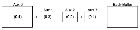
The method is illustrated with additive blending mode,
with example blending weights shown inside of the auxiliary buffers.

This method has the disadvantage of a fairly limited blur effect as it’s not practical to store a large number of previously rendered frames. The previous frames are also typically stored as ¼ or 1/16 sized buffers for memory considerations which decreases their resolution. This is typically acceptable as the blended frames are intended to look slightly blurred.

Another method is to store the current frame by blending it recursively on top of the previous one, in which case no extra work buffers are needed for the effect, and no resolution is lost for the previous frames.

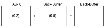
The image illustrates recursive blending,
with example blending weights shown inside of the buffers.

Note that in practice, the back-buffer doesn’t have to be used as a source texture as the example image would indicate. Rather, it’s more efficient to blend the auxiliary buffer directly on top of the existing back-buffer by alpha blending by using the following render states in the HLSL effect file.

AlphaBlendEnable = True;
SrcBlend = InvSrcAlpha;
DestBlend = SrcAlpha;

The pixel shader for the effect then becomes extremely simple.

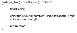
The HLSL sample code contains a pixel shader for the blur effect.

This method has a particular disadvantage as well. Although it is very easy to produce a heavy blur effect, large weights for the previous frame can produce a ghost image that remains on the screen without being blended out. This has to do with the precision of the buffers, which are typically only 8-bits per channel.

Thinking in 8-bits, if the auxiliary buffer contains a value 0/255 for the currently rendered frame, and the back-buffer contains a value 1/255 for the previous frame, the blending operation would then result into: 0*0.2 + 1*0.8 = 0.8. The resulting value of 0.8 would then be rounded back to 1. This means that even if the current frame is perfectly black, a ghost image from the previous frame would remain on the screen.

Bloom

There are different ways for designating the areas for blooming in the target scene. Apart from working with floating point buffers and implementing a real HDR, a high-pass filter can be used for extracting the bright areas from the regular scene, or the alpha channel (as mentioned in “Using the Alpha Channel”) be used for rendering the bloomed geometry separately.

The bloom filter typically consists of the following steps:

The image illustrates the stages and passes of the bloom filter.

The effect is typically started by extracting the bloom information into a smaller work buffer (Aux 1 here). A horizontal pass is then applied with a wide target buffer (Aux 2), and a vertical pass with a full-size target buffer (Back-Buffer).

The bloom effect is then achieved by sampling a number of neighboring texels for the current source texel in question, and assigning the texels further from the center decreasing blending weights. Separate horizontal and vertical passes are necessary for sampling a large enough number of texels, and avoiding a “star” artifact in the resulting image.

On the level of individual pixels, the passes look as follows:

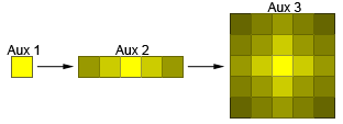
The image illustrates the horizontal pass in Aux 2 and the vertical pass in Aux 3.

A naïve implementation might sample each pixel at the texel center with the appropriate weight set for that texel. However, it is possible to optimize this process by enabling linear filtering for the source texture and sampling at texel boundaries (as mentioned in “Using the Hardware Filtering”), which allows for either a much larger number of samples to be taken to enhance the effect, or doing the same effect with less samples and thus optimizing its performance.

The following image illustrates this method:

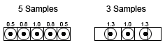
Bloom filters by sampling at texel centers and texel boundaries.

In the 3 sample method, the sampling points do not lie exactly at the texel boundaries. Rather, they take into account the blending weights for the each texel and the samples are then jittered so that the linear filtering automatically samples each texel with its relative correct weight comparing to its neighbor.

The correct offset between the texels can be calculated with the following formula.

Offset = Weight2 / (Weight1+Weight2)

The result of this sample has to be then normalized by multiplying it with the sum of the weights of both texels.

Weight = Weight1+Weight2

The calculation of offsets and weights should be done on the CPU, which leaves the vertex and pixel shaders as follows.

The HLSL code sample contains the input and output structures for the bloom effect.

The HLSL code sample contains the vertex and pixel shaders for the bloom effect.

Note that the sample offsets are packed into float4 texture coordinates for optimization. Typically the hardware may interpolate even float2 coordinates as full float4’s, thus using two separate variables of float2 would be wasteful, and it is instead better to pack all the information into as few variables as possible.

Image Perturbation

Perturbation of the rendered scene can be used for a multitude of effects such as simulating a daze, heat-shimmer or different blast waves.

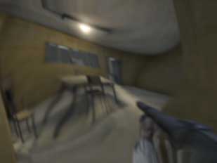
Battlefield 2: Special Forces featured an image perturbation effect
when the player was dazed by tear-gas. (The screenshot has been brightened for this article)

These effects are typically based on perturbing the source texture coordinates by using the sine and cosine instructions. In the case of the pixel shader model 1.4, these instructions are not available in which case they can be simulated by sampling a sine texture. The perturbation could also be moved to per-vertex level if using a highly tessellated target quad. In this case, at least a vertex shader model 2.0 would be required for using the sine and cosine instructions on the GPU. Alternatively, the vertices could be perturbed on the CPU for each frame.

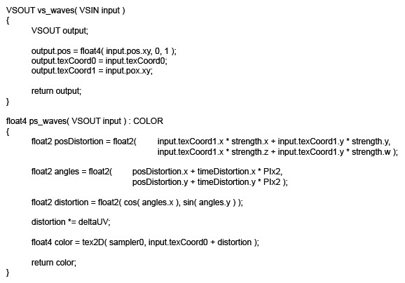
HLSL code sample for an image perturbation effect. Pixel Shader 2.0 required.

• deltaUV - pixel deltas as calculated at the beginning of this article.
• strength - 4 weights for tweaking the waviness of the resulting image.
• timeDistortion -2 time values for horizontal and vertical perturbation speeds, the values should loop within range 0-1.

Conclusion

Hopefully this article has both given some insight into the basics of post-processing, and highlighted some of the common problems experienced with it, while also giving ideas for solutions and optimizations for creating more efficient graphics engines and more advanced post-processing effects in general.

Many of the techniques mentioned here can be applied to a wide range of effects not covered in the article, and can hopefully serve as an inspiration for future work and adaptation for your own special-effects.