It's time to re-think A/B testing

In this article, I want to explain why we decided to completely change the way we perform A/B tests in Pixel Federation. I will be comparing the method we used before to the new method in context of A/B testing new features in F2P mobile games.

We usually test two versions of the game. Version A is the current version of the game. Version B is different with a new feature, rebalance or some other change. About a year ago, we were using the null hypothesis significance testing (NHST) known also as frequentist testing. Specifically, we used Chi-squared test for testing conversion metrics and t-test for revenue metrics like ARPU (average revenue per user) or ARPPU (average revenue per paying user). Now, we are using Bayesian statistics.

I will mention these main reasons why we switched from NHST to Bayes:

1. How to interpret the results?

The frequentist and Bayesian statistics have a very different approach to probability and hypothesis testing. So, the results we get from the same data are also quite different.

Interpretation of frequentist tests

The frequentist tests give us p-value and confidence interval as results. By comparing the p-value to predetermined alpha level (usually 5%) we conclude whether the difference is significant or not. This approach has been used for over 100 years and it works fine. But there is one big problem with p-values. A lot of people think they understand them, but only a few actually do. And this can lead to a lot of problems like unintentional p-hacking.

The reason is that p-values are very unintuitive. If we want to test that there is a difference between A and B, we must form a null hypothesis assuming the opposite (A is equal to B). Then we collect the data and observe how far are they from this assumption. The p-value then tells us the probability of observing data that are even further from the null hypothesis.

In other words, the p-value tells us the probability of getting an outcome as extreme as (or more extreme than) the actual observed outcome if we would have run an A/A test. This is the simplest description of p-value I know but it still seems too confusing.

I am not saying that complicated things are not useful. But in our business, we need also managers and game designers to understand our results.

So how do we interpret the result? If we get a result of p-value less than alpha, everything is fine. We make a conclusion that A and B are different which has clear business value. Everyone will be happy that we made a successful A/B test, and no one cares that they do not understand what the p-value actually means.

But what if we are not so lucky? It is hard to make a conclusion that has some value when we get p-value higher than alpha. We can see that on following example. This is the result from a Chi-squared test (calculated by Evan’s Awesome A/B Tools).

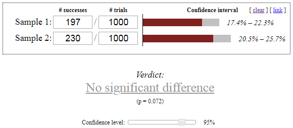
Not only we cannot say that one version is better, but we also cannot say that they are the same. Now, our only result is a p-value equal to 7.2%. We also have confidence intervals but that is not much help here since the confidence interval of difference would include zero. Now, the chances are that people from the production team will not understand what p-value equal to 7.2% means and if you somehow manage to explain it to them it can be even worse. Because who cares what is the probability of getting an outcome more extreme than the observed outcome under the assumption which is the opposite of what we hope for?

In this situation, it can be tempting to say “Well, 7% is quite close to 5% and it looks like there is an effect. Let’s say that B is better”. But you cannot do that, because p-values are uniformly distributed between 0 and 1 if there is no real effect. That means that if there really is no difference between A and B, there is an equal chance of p-value being equal to 7% or 80% or any other number. So, the only thing you can declare and keep some statistician’s integrity is that we do not have enough data to make any decision in the current setup of the test.

This is very disappointing because A/B tests are quite expensive. From the manager’s point of view, when we run a test for a few weeks and then analysts conclude that we know basically nothing it can look like a waste of time and money. I saw how this leads to frustration and unwillingness to do A/B tests in the future. And this is not what we want.

Interpretation of Bayesian tests

Bayesian approach solves this very well, because it gives us meaningful and understandable information in any situation. It does not operate with any null hypothesis assumptions and this simplifies a lot in terms of interpretability.

Instead of p-value, it gives us these three numbers:

E(loss|B) and E(uplift|B) are measured in the same units as the tested measure. In case of conversion, it is a percentage. Let’s see the result using the same data as before:

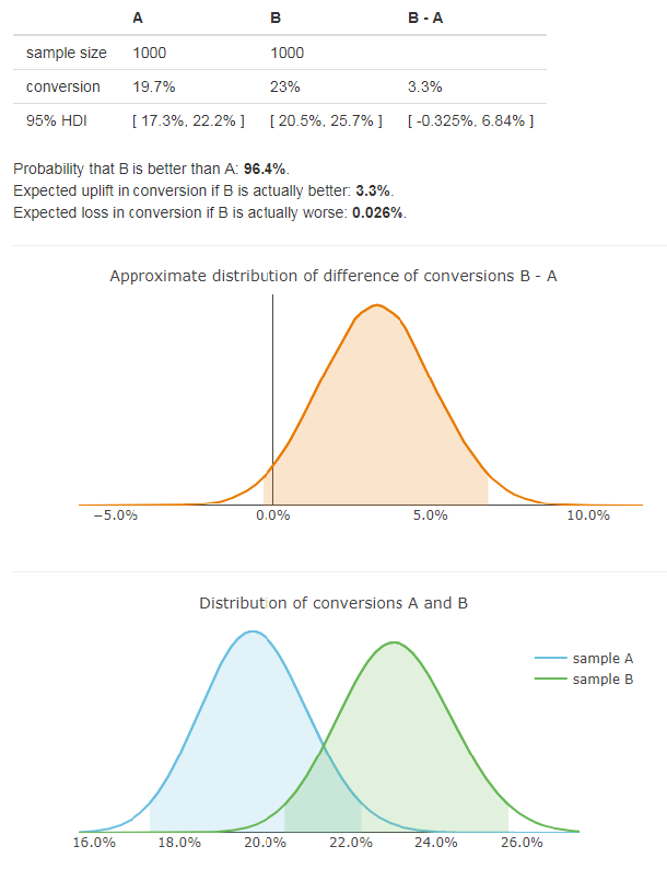
This result tells us that if we select version B, but it is actually worse (probability 3.6%) we can expect to lose 0.026% on conversion. On the other hand, if our choice is correct (probability 96.4%), we can expect to gain 3.3% resulting in 23% conversion. This is a simple result that can be well understood by both game designers and managers.

To decide whether to use A or B, we should determine a decision rule before calculating the results of the test. You can decide based on the P(B > A) but it is much smarter to use E(loss|B) and declare B as the winner only if E(loss|B) is smaller than some predefined threshold.

This decision rule is not as clear as with the p-value, but I would argue that it is a good thing. The “p-value < 5%” has become so wired in the brain of every statistician that we often do not even think about whether it makes sense in our context. With Bayesian testing we should discuss the threshold for E(loss|B) with game designers before running the test. Then we should set it to a number so low that we do not care if we make an error smaller than this threshold.

But even if the predefined decision rule does not distinguish between variations (because we do not have enough data, or we set the threshold too low), we can always do at least an informed decision. We can compare how much can we gain with the probability of P(B > A) and how much can we lose with the probability of 1 – P(B > A). This is the key advantage of Bayesian testing in business applications. No matter the results, you always get meaningful information that is easy to understand.

2. Sample size and setup of the test

So far, I have only mentioned issues about the understanding of the test results. But there is another very practical reason to use Bayesian testing regarding the sample size. The most often mentioned drawback of NHST is the requirement to fix the sample size before running the test. The Bayesian tests do not have this requirement. Also, they usually work better with smaller sample sizes.

Sample size in frequentist tests

The reason that fixing the sample size is required in NHST is the fact that the p-value is dependent on how we collect the data. We should calculate the p-value differently if we set up the test with the intention to gather observation from 10 000 players compared to the test where we intend to gather the data until we observe 100 conversions. This sounds counterintuitive and it is often disregarded. One would expect that the data itself are sufficient, but it is not the case if you want to calculate the p-values correctly. I am not going to try to explain it here since it is very well analyzed in a paper (see Figure 10) by John K. Kruschke and explained in even more detail in chapter 11 of his book Doing Bayesian Data Analysis. Another reason to fix the sample size is that we want some estimate of the power of the test.

This means that we must determine how many players will be included in the test before collecting the data and then evaluate the results only after the predefined sample size has been reached. But since we usually have no idea about the real size of the effect, it is very hard to set up the test correctly and efficiently. And because A/B tests are expensive, we want to set up them as efficiently as possible. This topic is very well covered in an article by Evan Miller. He clearly shows how “peeking” at the results before reaching the fixed sample size can considerably increase the type I error rate. And this completely invalidates the result. He also suggests two possible approaches to fix the “peeking problem”: Sequential testing or Bayesian testing.

Sample size in Bayesian tests

Bayesian tests do not require fixing the sample to give valid results. You can even evaluate the results repeatedly (which is considered almost a blasphemy with NHST) and the results will still hold. But I have to write this with a big warning! Some articles claim that Bayesian approach is “immune to peeking”. This can be very misleading, because it suggests the type I error rate is kept even if we regularly check results and stop the test prematurely when significant. This is just not true. No statistical method can do that if you have the stopping rule based on observing the extreme values. The fact is that Bayesian tests never kept the type I error rate bounded in the first place. They work differently. Instead, they keep the expected loss bounded. It is shown in this article by David Robinson that the expected loss in Bayesian tests is bounded even when peeking. So, the claim is partly true just be aware that being “immune to peeking” means one thing for NHST and something different for Bayesian tests.

I put the warning here in case you care specifically about type I error rate. In that case, the Bayesian testing may not be for you.

But I am convinced that type I error rate is not very important in our context. Sure, it is super important in scientific research like medicine. But the situation is different in A/B testing. In the end we always choose A or B. And if there really is no difference or the difference is very small we do not care that we made a type I error. We only care if the error is too big. So, in context of A/B testing it makes much more sense to bound the expected loss instead of type I error rate.

On top of this, there is another practical advantage in Bayesian tests. It usually requires considerably smaller sample size to achieve the same power compared to NHST. This can save us a lot of money, because we can make decisions faster.

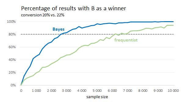
Following plots show simulations of conversion tests. We simulated 1 000 Chi-squared tests and 1 000 Bayes tests for each sample size and calculated the percentage of tests that correctly declared B as a winner. That tells us the approximate power of the test with a specific sample size.

We can see that the sample size required to get 80% power is significantly lower for Bayesian tests. It is less than half. On the other hand, if we plotted the situation where the conversion of A and B is the same, the NHST would have better results (95% for any sample size).

For Chi-squared test, we used alpha equal to 5%. The Bayesian test declared B as a winner when the expected loss was lower than 0.1%.

How it works in practice

After talking about the reasons for the change I should also mention how we use it in practice. For now, we are using two separate Bayesian models for two different types of tests. Without detailed explanations (which would need a separate article), I will just list what we use right now.

Instead of Chi-squared test, we use a model that assumes that the conversion rate has Bernoulli distribution. All the formulas are from following sources:

For revenue data, we have an extension of the conversion model. It separately estimates the conversion rate with the Bernoulli distribution and then the paid amount using the Exponential distribution. I implemented it based on this paper:

Code available with Kruschke’s book was also very useful in understanding the Bayesian statistics. I used parts of it to calculate the highest density intervals:

Using these sources, I implemented A/B test calculators in R. You can give them a try here:

Summary

Using Bayesian A/B testing, we can now carry out tests faster with more actionable results. Let me summarize the advantages below:

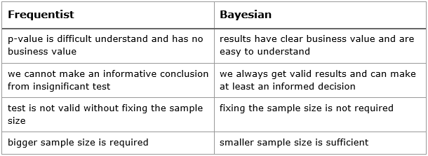
But what are the disadvantages and why is it not used more often? In my opinion, the main reason is that it is far more complicated to implement compared to traditional NHST tests which can be calculated using one function in Excel. Another reason some are hesitant to use Bayesian approach is the prior distribution. Prior and posterior distributions are key elements of Bayesian statistics. You have to determine the prior distribution before doing any calculations. In Pixel Federation, we are currently using non-informative priors for A/B testing purposes.

In conclusion, I want to emphasize that I am not claiming that frequentist statistics is generally inferior to Bayesian. They are both useful for different purposes. In this article, I wanted to argue that Bayesian approach is more appropriate in business applications.

If you happened to face similar problems and solved them differently or you used Bayesian statistics and have some experience you wanted to share, please let me know.

Sources