Refractive Texture Mapping, Part One

This article presents, in two parts, a detailed implementation of refractive texture mapping for a simple water wave simulation using directional sine waves applied to a flat polygonal mesh. It is assumed that the reader is familiar with the 3D transformations pipeline, simple vector algebra, surface modeling using polygons, as well as UV coordinates for texture mapping.

This article is better suited for console development, but for sake of clarity, the sample program was implemented in a Pentium 300 with a 3D graphics card, and using DirectX 7. Even though DirectX 7 has its own implementation of one of the mapping techniques described in this article (sphere mapping), DirectX 7 was only used to transform and render the final polygons in the sample program. All the UV coordinate calculations, perturbations, normal calculations, and so on, were done internally by the program. It's also important to note that the hardware did all the transformations, and all the calculations described here are in world space. However, these calculations can be easily done in object space if necessary as described further.

Motivation

Last year I started to play around with a particular texture mapping technique called sphere mapping. As I went further in my research, I found out that sphere and refractive texture mapping were similar. At the end, I started to be interested in writing a real-time water wave application using refractive texture mapping. Meanwhile, I also found out that the literature about the subject was not too clear. Most of the papers, articles, and books either described the techniques too briefly, missing a number of details, or dove into things such as fluid dynamics.

In this series of articles, I'll present some experiments I did with sphere and refractive texture mapping, as well as few tricks I learned to speed up the code, without compromising the quality of the final rendering too much. The first part will focus on using sphere mapping to simulate curved-surface reflections, and in part two I will describe how to use refractive texture mapping to simulate water refraction, complete with optimizations and a sample program.

Sphere Mapping

Sphere mapping is a technique used to simulate reflections in curved surfaces. There is a really good discussion about sphere mapping in Real-Time Rendering by Möller and Haines, and also in the DirectX 7 SDK documentation. Here I've presented a simplified version of the technique that can be done basically in two steps. First, the reflected rays from the camera's position to the object are computed. Second, the reflected rays' values are interpolated as texture coordinates. Note that a special texture is normally used for the final rendering.

By looking at the figure above (Figure 1), the reflected ray is computed by the formula:

In the particular case of a polygonal mesh, the surface normals (N) are the vertex normals. A simple way of computing the vertex normal is by averaging the surface normals of all polygons sharing this vertex. The incident rays (V) are the vectors between the mesh vertices and the camera position.

Once the reflected rays are computed, their results need to be transformed in texture coordinates. As in 3D space, the reflected ray has three values (X, Y, Z) and the texture mapping is a 2D entity, the values need to be transformed in some way to generate the final UV coordinates. There are several ways of transforming the reflected ray values in UV coordinates. An easy an simple way is just to ignore one of the values (in my particular implementation, the Z value) and interpolate the remaining two values as UV coordinates. This approach is reasonably fast and generates good results. After the UV coordinates are stored in the mesh data structure, the polygons are sent to the hardware to be transformed and rendered.

Even though the process is simple, there are few details to be considered for the implementation, specially if the target machine is a console. Let's look at pseudocode below to see these details.

Listing 1. Sphere mapping

//main loop
vertex_current = (VERTEX_TEXTURE_LIGHT *)water->mesh_info.vertex_list;
for (t0=0; t0mesh_info.vertex_list_count; t0++,

{

}//end main loop

First, all the coordinates are assumed to be in world space. This is because the mesh vertices are in world space (in the sample program), and the vectors from camera to the mesh vertices (incident rays) are also in world space. In case you need the object (mesh) to be in object space, you must transform it into world space before applying the calculations. Otherwise you must transform the incident rays back to object space. Whichever is more convenient for you depends on the hardware and the application.

Second, the mesh normals need to be computed and normalized before the loop above starts. The sample code uses the simple average surface normals approach. Third, all the other vectors need to be normalized to avoid roundoff errors, and for the final interpolation. Also, looking at how the incident ray is being computed in the code above, you can see that it's inverted. This is for debugging purposes. The implementation can display the rays (see Figure 2), and if they were in the right direction, they would pierce the object. The inverted incident ray does not cause any problems, it just hits the map inverted. Finally, as the components of each normalized reflected ray vertex are going from -1.0 to 1.0, by simple algebra they can be linearly interpolated as:

If the reflected ray is normalized and the texture coordinates come from this vector, the vector will hit the map in a shape of a sphere. For this reason, a special texture is normally used. The texture needs to represent a full view of the environment distorted as if seen through a fish-eye lens. Figure 3 is an example of this type of texture.

In water simulation, sphere mapping can also be used simulate water reflections. Also, in the code above there are couple of vector normalizations, which might not be too efficient on some platforms. However, most console hardware can perform vector normalization reasonably fast. Also, the spherical texture for water simulation, is really not a requirement. If the application does not need to generate a reflection of the environment, graphic artists can experiment with different types of textures until good results are achieved.

Perturbations

The water mesh is implemented as a flat polygonal mesh using the left-hand coordinate system, where the Y-axis represents the up dimension and the Z-axis points away from the viewer. This mesh is divided in n slices in either dimension specified by the user. The figure below shows the top view of the mesh as if it's been divided in three slices.

Sphere mapping or refractive texture mapping is not too interesting over a flat mesh, especially for simulating water. Taking this fact into account, it's necessary to perturb the mesh.

There are several ways of perturbing the mesh to look like water, some faster and some slower. A very efficient way is by using the array approach described by Hugo Elias and Jeff Lander ("A Clean Start: Washing Away the Millennium," Game Developer, December 1999). However, the array approach only simulates approximations of ripples on the mesh. If the application needs to perturb the mesh with a constant directional wave, or a combination of directional waves, the array approach cannot be used. Another method is to use a spring model, modeling the flat surface as a set of two dimensional springs, which can produce very realistic effects. Lastly, we can simply use sums of sine or cosine functions which creates very good results. For the sake of simplicity, the sample program explained here implements perturbations using sums of sine wave functions.

Sine Waves

In order to understand how the sample program perturbs the polygonal mesh using sine wave sums, let's quickly review some properties of sine wave functions.

In 2D space (X, Y) as function of X, sine waves can be written as:

The amplitude (a) is how big the wave is because it multiplies the whole function. The wave number (k) is related to the wave frequency: the smaller this number is, the greater the frequency and vice versa. The phase shift shifts the wave to either a positive or negative direction of the X-axis. In terms of animation, we can use the time as a phase shift to make the waves move each frame.

In 3D space, the sine wave equation can be extended to (using the left-hand coordinate system):

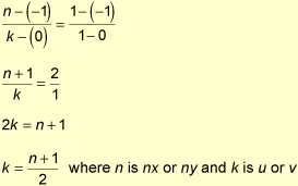
Equation 4 is a straightforward extension of Equation 3 for 3D space. The only part that needs special attention is the wave directional vector components (i, j). In this case, they define in which direction the wave is traveling on the XZ plane. As an example, let's write the wave equation as if the wave is traveling 45 degrees (p/4 radians) in respect to the X-axis.

If we project the wave directional vector (unit vector) on the X- and Z-axis, by simple trigonometry the components can be computed as:

and

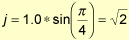
So the equation for this example can be written like:

Ripple Equation

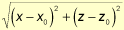
To generate ripples on the mesh, a similar equation is derived from the sine wave equation combined with the circle equation. By looking at the Figure 6, the circle equation can be written as:

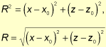
If the sine wave equation is applied to the radius, ripples are created; therefore the final ripple equation can be written as:

Perturbations Combined

If each perturbation function (ripple or directional wave) is written as wk(x, z), the final mesh perturbation is the sum of all functions such as:

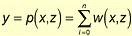
(Equation 6)

Implementing of all these equations (4, 5, and 6) together is straightforward. The program just loops though all vertices of the mesh applying equation 4 or 5 (depending on the type of perturbation) to the X and Z mesh values. Then it sums the Y coordinate results of each perturbation and stores the final result back on the mesh vertex data. It is important to note that as the original mesh was created as flat rectangular mesh divided into slices, the finer the mesh (that is, the more polygons), the more accurate the waves are. However, more calculations are necessary. The pseudocode in listing 2 shows how these sums of perturbations can be implemented, as well as the perturbation data structure used in the sample program.

Listing 2. Sums of wave functions applied to the mesh

//pertubation data structure example
typedef struct _water_perturbation
{

}WATER_PERTURBATION;

vertex_list= (VERTEX_TEXTURE_LIGHT *)water->mesh_info.vertex_list;

for (t0=0; t0mesh_info.vertex_list_count; t0++)
{

First Simulation Using Sphere Mapping

If sphere mapping is applied to a perturbed polygonal mesh, a very interesting effect can be achieved (Figures 7 and 8 show the results, Figure 9 shows the textures used). The implementation is a combination of the two techniques explained before, plus the vertex normal calculations, because the mesh deforms each frame. Finally, when the perturbation values are tuned (amplitude, frequency, velocity, and so on), it's important to use small amplitudes for the waves. In tall waves the textures stretch too much, creating undesirable effects. The code for the render function is shown in Listing 3.

Listing 3. Render function using sphere mapping

result water_render (WATER *water)
{

}

Next time, in part two of this article, I will dive into refractive texture mapping for simulating water refraction. I'll also provide a second simulation as well as some optimizations and the sample application.

References

Möller, Tomas, and Eric Haines. Real-Time Rendering. A.K. Peteres, 1999. pp 131-133.

Direct X 7 SDK Help (Microsoft Corp.)

Serway, R. Physics for Scientists and Engineers with Modern Phyisics, 4th ed. HBJ, 1996. pp. 1023-1036.

Ts'o, Pauline, and Brian Barsky. "Modeling and Rendering Waves: Wave-Tracing Using Beta-Splines and Reflective and Refractive Texture Mapping." SIGGRAPH 1987. pp. 191-214.

Watt, Alan, and Fabio Policarpo. The Computer Image. Addison-Wesley, 1997. pp. 447-448.

Watt, Alan, and Mark Watt. Advanced Animation and Rendering Techniques: Theory and Practice. Addison-Wesley, 1992. pp. 189-190

Harris, John W., and Horst Stocker. Handbook of Mathematics and Computational Science. Springer Verlag, 1998.

PlayStation Technical Reference Release 2.2, August 1998 (Sony Computer Entertainment)

Elias, Hugo. http://freespace.virgin.net/hugo.elias/graphics/x_water.htm

Lander, Jeff. "A Clean Start: Washing Away the New Millennium." Game Developer (December 1999) pp. 23-28.

Haberman, Richard. Elementary Applied Partial Differential Equations, 3rd ed. Prentice Hall, 1997. pp. 130-150.

Graff, Karl F. Wave Motion In Elastic Solids. Dover Publications, 1991. pp. 213-272.