Daily news, dev blogs, and stories from Game Developer straight to your inbox
Sponsored By
Featured Blog | This community-written post highlights the best of what the game industry has to offer. Read more like it on the Game Developer Blogs.
Introduction to Inventory-Aware Pathfinding
Solving planning and pathfinding at the same time can save you a lot of time. It is the case of Inventory-Aware Pathfinding where we want to solve pathfinding in a map constrained by the items brought by the agent (e.g., keys to open locked doors).
9 Min Read

Everybody know what pathfinding is. I don’t think I have to explain to a game developers audience why pathfinding is so important in games. If something in your game is moving not in a straight line, then you are using some kind of pathfinding.
What is less evident is that pathfinding is the only place in which “searching” is generally accepted. Except for GOAP and other planning-based techniques, the big part of the NPC’s decision-making techniques are reactive-based.
This is not a bad thing. Reactive techniques are an amazing design tool. However, this raises a question. Why is this? Mainly because of computational limits – full-fledged planning still requires an impractical amount of time – but also because of design unpredictability. The output of planning decision-making techniques is hard to control and the final behavior of the agent could be counterintuitive for the designers and, at the end, for the players.
Why can pathfinding play a role in this? Because it is possible to embed in it a minimal, specialized, subset of planning, especially if these planning instances require spatial reasoning. A common example is solving a pathfinding problem in which areas of the map are blocked by doors that can be open by switches or keys sparse around on the map. How can we solve this kind of problems?

We can choose between two paths. We can try to reach the goal (King) without the key, or take the key and go through the door. With just 1 key, this problem is quite easy.
The Keys/Doors Pathfinding Problem
Look at the example above. There are two possible paths: in the first one, the agent do not require to click the switch and, in the second one, it needs to go to the switch, open the door and then pass through it. The optimal path, in this case, is easy to compute but we can clearly see that it depends on the start, the goal, but also on the key and door relative position. In a formal way, we want the shortest path among one of the possible path:
Path 1. The path between S and G assuming the door is closed. In math, D(S,G).
Path 2. The path passing through the door. In math, D(S,K) + D(K,D) + D(D,G). Being careful that we assume the door closed for D(S,K) and the door open for the other distances.
Because D(K,D) is fixed on the map and we can precompute it, we can solve this problem with just 3 pathfinding instances ( D(S,K) , D(D,G) , D(S,G) ), compare the result and chose the faster path. In the above example "Path 1" is 13 steps long and "Path 2" is 13 steps too. Put the agent one step forward in the green line direction and "Path 1" will be the faster path; put the agent one step forward in the red line direction and the other "Path 2" becomes the best path.

7 of the 13 total paths possible with 2 keys and 2 doors. It is already a mess. With 3 keys we will have way more problems.
However, now we will try to add another key and another door to the map. Now, the number of possible alternative paths increase to 9 paths. In fact, we can choose between:
A path that ignores every switch and door.
A path that uses only (K1, D1).
A path that uses only (K2, D2) .
6 paths who use both (K1, D1) and (K2, D2) .
About point 4, why 6 paths? It easy to verify that there are exactly 6 ways to arrange K1, D1, K2 and D2 with the constraint that Ki appears before Di. We can list these permutations:
K1, K2, D1, D2
K2, K1, D1, D2
K1, K2, D2, D1
K2, K1, D2, D1
K1, D1, K2, D2
K2, D2, K1, D1
These are 13 pathfinding instances. 5 if we assume that every "internal path", the paths between every key and door to every other key and door, is known at runtime.
Unfortunately, the number of paths in a map with n keys-doors increase faster than factorial. In fact, we need to test every valid path in a graph like the one shown in the image above. To give you an idea, this is the number we can obtain if we sum the number of permutations in which the i-th key appears before the i-th door for every subset of {K1D1, ..., KnDn}. This number in between 2^n times n! (n factorial) and 2^n times 2n! (2n factorial). A huge number, indeed.
Though, we are clearly doing a lot of extra work. Why do we need to compute a priori every possible combination of paths? Why have I to take into account a switch or a door that is miles away from my current position? Why have I to look for combinations of keys and doors that are “clearly” bad?
In fact, we don’t. If we apply the same pathfinding reasoning to the “key-door space”, if we perform some kind of spacial reasoning, if we search for the path at the same time we search for a solution to the key-door problem, we can cut a lot of computation.
A simple Inventory-Aware Pathfinding
The first intuition is the following. Instead of looking at keys and doors as a particular state of the map, we can start considering keys and switches as portals to a different map in which the corresponding door doesn’t exist anymore.

The same example as before. However, this time, we use the item-level representation. As you can see there are no more doors and the keys act like a “portal” between levels.
We can look back at the first example. Instead of a bidimensional map with a door that can be open or closed, we have a “3D map” without doors. Each “level” (we can call them item-levels) of this map represent the state of the world when the agent carries a particular set of keys. For instance, the Level 0 in the image represents the world as if we have no key. Level 1, instead, represents the world as if we have taken the key.
At this point, we can forget about the doors and use this expanded map as a traditional pathfinding problem in which:
The state in the search algorithm is expanded in order to take into account the “3D item-level position”. That is, from storing just the position in the 2D space <x,y>, to the 3D expanded state <x,y,k1,...,kn> where every ki can be 0 or 1 depending on the fact that we are on a level in which we have the i-th key.
The keys on the map are just “stairs” who allows us to travel between the item-levels. If we assume that we cannot drop a key we can treat this “stairs” as one-way only.
We have now multiple goals. In fact, we don’t care on which level we reach the goal, all this state represent the exact same position in the real 2D space.
We can now apply any pathfinding algorithm to this problem. However, we have not removed the exponential complexity. In the worst case, in fact, we need to search every item-level and their number is 2^n where n is the number of keys. Because levels are searched in the same pathfinding algorithm, we avoid searching the same item-level multiple times cutting off the factorial complexity we have seen before. A huge cut, indeed.
Are we in the right direction?
The algorithm above is quite simplistic but it give us several benefits:
With 0 keys on the map, this algorithm is exactly equivalent to a standard pathfinding algorithm. No overhead, no additional complexity. Nothing.
If a key is not encountered in the search horizon of the algorithm it does not affect the performances at all. This happens a lot if we are searching for small paths. In this case, the search algorithm is not affected by keys that are ten miles away from the goal.
At the same time, there are many drawbacks that we still need to address.
It searches extensively an exponential number of levels, this is a problem especially when there is no path to reach the destination. In this case, the algorithm is forced to search everything before it can assure that there is no path.
The heuristic does not take into account keys and doors. This means that in those level in which the goal is not reachable (and thus, we need some other key) the search is driven in the wrong direction (the goal direction) for no purpose. It can waste a lot of precious time.
Another consequence of Point 2 is that item-levels are explored prioritizing “fewer keys”. This is a good strategy in general but if many keys are needed in order to reach the goal we waste a lot of time searching in “not promising” levels.
Keys add computational cost regardless of their potential utility. If keys are “dense” around the starting point we a rapid explosion in the time required in order to reach a solution. This sensitivity of the algorithm respect starting position and keys distribution may be problematic in some cases.
The algorithm described in this paper (a joint work with Stavros Vassos and Sebastian Sardina) shows that this base solution can achieve some practical results on constant cost grid maps if the number of keys on the map is in a reasonable range (around 6-7 keys). In the paper, we used a slightly modified version of Jump-Point Search and using all the saved computation power for solving the key-door problem. However, we want to do more.
This is only the start of the journey. There is still a lot of wasted time we can save with the right techniques. But we will talk about that at a later time.
I'm Davide Aversa, a Ph.D. student at "La Sapienza" University of Rome and small game developer by myself. My research focus is on Artificial Intelligence and Smart Pathfinding for videogames. If you have any question, let me know!
Read more about:
Featured BlogsAbout the Author(s)
You May Also Like