Originally posted here.

Overview of Inverse Kinematics System

One of the most popular solutions to the Inverse Kinematics problem is the Jacobian Inverse IK Method. This method was largely used in robotics research so that a humanoid arm could reach an object of interest. This method is very powerful, but also has the potential to be computationally expensive and unstable if it is not understood well.

As a recap, any IK problem has a given articulated body (a set of connected limbs with lengths and angles). The end effector (the position of the endpoint of the final limb) has a start position with a goal position. It might have other goals, such as angles.

Jacobian methods have three main steps from a top-down perspective:

1. Find the joint configurations: T

2. Compute the change in rotations: dO

3. Compute the Jacobian: J

1. Find Joint Configurations

Let’s start with the math required to get from the initial pose to the target position for the end effector.

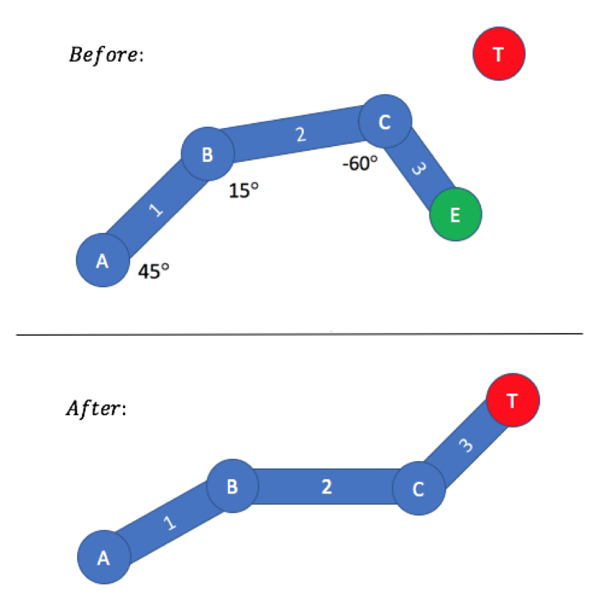
Assuming all the joints are revolute, then O is a pose vector which represents the initial orientation of every joint. T is the pose vector which represents the final orientation of every joint, such that the end effector reaches its target position. dO is the vector which represents the change in orientation for each joint, such that the articulated body reaches T from O. For example, O would be (45°, 15°, -60°) in the Figure below.

As you can see, only the initial pose vector O is known. We want to find T so that the end effector can reach the target position. To do this, we need to find dO first.

Jacobian methods use an iterative approach in calculating dO, similar to the Gradient Descent Method. We find iterative solutions to dO, where each successive solution is closer to the final answer than each preceding solution. Each successive solution finds the local minimum of the error. As such, to leverage the iterative approach, we need to modify the above equation:

Where h is just a simulation step that can be tuned. A good starting value for h might be 0.01 — potentially even as low as 0.000000001. Make sure to test values that make the IK system most stable and less likely to explode. In code, this might look like so:

/* Step One */
void JacobianIK(O) {
    while( abs(endEffectorPosition — targetPosition) > EPS ) {
        dO = GetDeltaOrientation();
        O += dO * h; // T=O+dO*h
    }
}

The code above continues to loop/iterate on updating the O vector with the calculated dO. First you calculate dO. Then you multiply dO by some simulation step, h, of your choosing. Then that product is added to the current configuration vector, O. You repeat this until the endEffectorPosition is close enough to the targetPosition, as defined by some EPSILON value of your choosing. That’s it for Step 1!

2. Compute Change in Orientation

At this point, we still need to find dO. A Jacobian matrix will be essential in calculating the iterative values for dO, using the following equation:

Where J is the Jacobian and V is the change in spatial location. V is merely the difference between the end effector position and the target position: V = T-E. And the Jacobian is merely a matrix which represents the relationship between the position of the end effector and the rotation of each joint.

For now, let’s treat the Jacobian matrix as a black box, and continue with the mathematical equations we need to find dO. To find dO, we need to invert the Jacobian matrix to get us this equation:

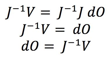
From here, we have an equation that allows us to find dO. It’s simple enough to calculate V = T-E. Afterwards, we also need to calculate the Jacobian and then invert it. As you will see, calculating the Jacobian is not extremely difficult; however, inverting the Jacobian matrix can be computationally expensive. Not only that, but the Jacobian matrix may not necessarily be square and thus an inverse solution may not even exist. This is confirmed by the properties of Invertible Matrices from College-Level Linear Algebra.

A rough approximation to the Jacobian Inverse that works in many simple cases is replacing the Jacobian Inverse with the Jacobian Transpose:

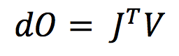
The Jacobian Transpose always exists, as opposed to the Jacobian Inverse. It is also less computationally expensive, which means that the performance will be faster. Additionally, the Jacobian Transpose is easier to implement than the Jacobian Inverse.

Now we have a simple equation that computes dO. This can be shown in code as follows:

/* Step Two */
Vector GetDeltaOrientation() {
    Jt = GetJacobianTranspose();
    V = targetPosition — endEffectorPosition;
    dO = Jt * V; // Matrix-Vector Mult.
    return dO;
}

The code above will calculate dO. First you calculate the Jacobian Transpose. Then you calculate V = T-E. Finally, you multiply the Jacobian Transpose and V, using matrix vector multiplication. And that’s all there is for Step 2!

3. Compute Jacobian

At this point, we still need to calculate the Jacobian Transpose. Let’s look at the Jacobian in mathematical form, to really understand what is going on. The Jacobian matrix is a function of the current pose as follows:

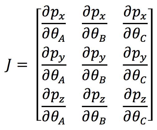
Each term in the Jacobian matrix represents how a change in the specified joint angle effects the spatial location of end effector. For example, the first term shows how much the end effector position would change along the X-axis, if Joint A’s angle is changed by a differential amount, such as 0.00001. Along the same lines, the first column shows how much the end effector position would change in X-Y-Z coordinate space, if Joint A’s angle is changed by a differential amount.

Calculating each term can be solved analytically or numerically, but using the analytical form is simple enough:

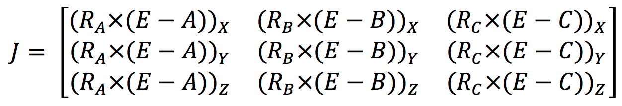
The above is the calculation for each entry. The representation can be simplified by having each entry be a vector instead of a scalar, as follows:

R_A is the axis of rotation of joint A. E is the position of the end effector, as before. And A is the position of joint A. The same logic follows for the second and third columns in the Jacobian Matrix. Now we have all the mathematical elements to compute the Jacobian Matrix, this is what it would look like in code:

/* Step Three */
Matrix GetJacobianTranspose() {
    J_A = CrossProduct(rotAxisA, endEffectorPos — jointAPos);
    J_B = CrossProduct(rotAxisB, endEffectorPos — jointBPos);
    J_C = CrossProduct(rotAxisC, endEffectorPos — jointCPos);

    J = new Matrix();
    J.addColumn(J_A);
    J.addColumn(J_B);
    J.addColumn(J_C);

    return J.transpose();
}

The first line of code calculates the first column of the Jacobian matrix. The second line of code calculates the second column of the Jacobian matrix. The third line of code calculates the third column of the Jacobian matrix. Let’s take a look at the first line of code, which relates to joint A. The first line of code is a cross product of two terms. The first term is the rotation axis of joint A. The second term is the difference between the end effector position and the position of joint A. The second and third lines of code follow the same logic for joints B and C. Now, all we do is combine all three columns to form the whole Jacobian. And finally, we return the matrix transpose of the Jacobian. That’s all there is for Step 3!

Final Notes

Keep in mind that this articulated body in the figure above has three joints, so the Jacobian had three columns. But if you have more joints, then you have more columns in the Jacobian. One column per joint in the Jacobian.

You might want to give this article a second read to get a better understanding of the mathematics involved. If not, feel free to look through the code excerpts in the article to get a simple sense of how to code up the Jacobian IK. Remember, it just takes three steps to implement the Jacobian IK.