We need to use movement prediction in our games more often than we might expect. We, as humans, predict the future position of objects all the time, and we act accordingly to that prediction. For example, when we want to catch a moving ball, we do not run to the place where it is currently in the air or on the ground. Instead, we naturally predict where the ball will be in a few seconds and move toward that predicted position. Based on our prediction skills we can catch the ball easily, or not so easily if our prediction was wrong.

Here are the examples of calculating predicted movement in a game:

In general, if we want to predict the movement of an object, we need to execute some form of physical simulation. The ideal situation would be if we could simulate the whole physical world for the needed time in the future. In most cases, because of the limited computing power, this is not (yet!) reasonable. However, depending on our needs, we can perform a simplified simulation to get the predicted state of the single object in the future.

In this article, I would like to describe three different scenarios of how we typically use prediction in games:

Nevertheless, we still need to remember that this is a prediction. We are not running the full physical simulation. Rather, we want to compute the most probable state of the object in the future.

To perform our predictions as a form of physical simulation, we need the basic physical quantity for the kinematic object: a velocity [1]. In general, the velocity is a rate of change of position in respect to time and is expressed using a derivative:

However, for our prediction needs, we can use the formula for the velocity during the constant movement, without referring directly to the derivative:

where  is the position displacement (from point  to ) and  is the elapsed time (from  to ).

Velocity is a vector quantity, which has a direction and a length. The length of a velocity vector is a scalar value and can be called speed.

Character

Our main concern for the character is the prediction for the short amount of time in the future - usually less than 1 s. This is the basic case for the prediction, where we make a few assumptions:

We start with the formula for the constant velocity from the previous section:

But this time we assume that , , and  are known variables and  is unknown.

We multiply both sides by :

Then, we move  to the left side:

Finally, we swap both sides of the equation:

and we get the final formula, where  is the current position of the character,  is the character’s velocity,  is the time of the prediction, and  is our predicted position in the future.

This formula has a natural geometrical explanation. The object moves with a constant linear movement, so we are moving the point along the velocity vector  from the point  to the point .

Below you can find the code in Unity Engine™ with a straightforward implementation of the final formula:

Vector3 LinearMovementPrediction(Vector3 CurrentPosition, Vector3 CurrentVelocity, float PredictionTime)
{
    Vector3 PredictedPosition = CurrentPosition + CurrentVelocity * PredictionTime;
    return PredictedPosition;
}

In navigation, the process to predict the position in the future is called “dead reckoning” [2] and it uses this formula as the basic computation technique.

This is also a simple formula to predict the movement of a character in multiplayer games while waiting for a new network data to arrive [3, section ‘Display of Targets’].

On the image below, we have an example with a geometrical description for this prediction scenario:

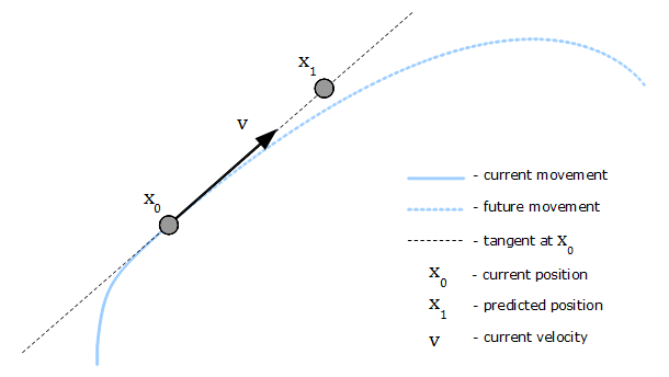
The blue curve marks the movement of the object (dashed blue line is the future movement). Velocity is the derivative of position function, so it lies on a tangent at the point  [4, section 'Kinematic quantities']. Since we are predicting position along the velocity vector, we can observe how a longer prediction time  will cause the predicted position to diverge from the real position in the future. A shorter prediction time  gives a better approximation.

Acceleration

There are situations when we want to consider acceleration in our prediction. In such cases, instead of assuming the constant velocity, we will assume the constant acceleration during the prediction period:

where  is the initial velocity,  is the final velocity, and  is the prediction time.

The formula for the predicted position  with the constant acceleration  is given by

As we can see, when there is no acceleration (), this formula still gives the same prediction result as the equation from the previous section.

The formula can be easily explained using the graph below for one-dimensional movement:

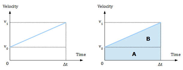
The graphs show a relation between velocity and time. In other words, it shows how velocity (a blue line) changes over time. When the graph is given in such a way, the area under the velocity line (marked with a blue color) is the distance traveled by the moving object [1, section ‘Instantaneous velocity’]. We can calculate that area as a sum of two figures: a rectangle A and a right triangle B.

Using notation for the areas with the initial distance  and the final distance  traveled by the moving object, we get the formula:

The area of the rectangle A is:

The area of the right triangle B can be computed as the half of the upper rectangle:

Because the acceleration is given by  , so . Using that, we can change the equation above to:

Finally, substituting for A and B in the first formula for  we get:

By renaming variables  to  and  to , we obtain the formula for the predicted position  given at the beginning of this section:

Projectile

In the case of projectiles, we are interested in the much longer time of our prediction. Additionally, we want to track the projectile when it bounces off other objects.

To perform this prediction, we need to execute a simulation loop and check for collisions in every step. We will assume simple ballistics physics for the projectile moving as a point [4, section ‘Uniform acceleration’]. Below is the code with the implementation in the Unity Engine:

Vector3 PredictProjectileMovement(Vector3 InitialPosition, Vector3 InitialVelocity, float TimeToExplode)
{
    float Restitution = 0.5f;
    Vector3 Position = InitialPosition;
    Vector3 Velocity = InitialVelocity;
    Vector3 GravitationalAcceleration = new Vector3(0.0f, -9.81f, 0.0f);
    float t = 0.0f;
    float DeltaTime = 0.02f;

    while (t < TimeToExplode)
    {
        Vector3 PreviousPosition = Position;
        Vector3 PreviousVelocity = Velocity;

        Position += Velocity * DeltaTime + 0.5f * GravitationalAcceleration * DeltaTime * DeltaTime;
        Velocity += GravitationalAcceleration * DeltaTime;

        // Collision detection.
        RaycastHit HitInfo;
        if (Physics.Linecast(PreviousPosition, Position, out HitInfo))
        {
            // Recompute velocity at the collision point.
            float FullDistance = (Position - PreviousPosition).magnitude;
            float HitCoef = (FullDistance > 0.000001f) ? (HitInfo.distance / FullDistance) : 0.0f;
            Velocity = PreviousVelocity + GravitationalAcceleration * DeltaTime * HitCoef;

            // Set the hit point as the new position.
            Position = HitInfo.point;

            // Collision response. Bounce velocity after the impact using coefficient of restitution.
            float ProjectedVelocity = Vector3.Dot(HitInfo.normal, Velocity);
            Velocity += -(1+Restitution) * ProjectedVelocity * HitInfo.normal;
        }

        t += DeltaTime;
    }

    // Return the final predicted position.
    return Position;
}

We will explain the code given above in the following three subsections: Simulation loop, Collision detection, and Collision response.

Simulation loop

The choice of the time step (DeltaTime) for every iteration depends on our requirements for accuracy. Typically, this will be the same value as the time step for our physics engine (in Unity Engine the default value is 0.02 s).

At the beginning of the loop, before evaluating our movement equations, we store position and velocity in PreviousPosition and PreviousVelocity variables. This is required to perform collision detection.

We are considering only gravitational acceleration, which is constant during the whole movement. Because of that, we can use the formula from the previous section to compute the new position after a given time step:

Position += Velocity * DeltaTime + 0.5f * GravitationalAcceleration * DeltaTime * DeltaTime;

Similarly, the new velocity is calculated using acceleration:

Velocity += GravitationalAcceleration * DeltaTime;

Collision detection

The essential part of the loop is the test for collisions, which is described in the image below:

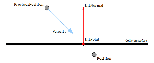
We use position from the previous step (variable PreviousPosition) and the newly calculated position (variable Position) to test if the line segment between them hits any objects. The collision test is performed by the Unity Engine method Physics.LineCast:

Physics.Linecast(PreviousPosition, Position, out HitInfo)

If there is a collision, the method returns true and stores the result in HitInfo:

Having that data, we can recalculate position and velocity at the point of collision.

The velocity is recomputed first to get the precise value at the HitPoint. The variable HitCoef has a value between 0 and 1, and is the ratio of the HitInfo.distance to the total length of the line segment. We recompute the velocity using the same movement equation but scaling the last component with the HitCoef. In this way, we scale the DeltaTime to the moment of collision and obtain the value of the velocity at the collision point.

The new position is simply the point of impact.

Collision response

Finally, we are ready to bounce the velocity according to the impacted surface. We use the HitNormal and coefficient of restitution (how strong the bounce should be) [5]. The value of Restitution should be between 0 and 1. If the Restitution variable is 1, there is a perfect bounce, and no energy is lost at the collision. If the Restitution is 0, then the whole energy is lost, and the velocity along the hit normal is canceled entirely.

Calculation of the bounced velocity (after the impact) is described in the image below and the following text derives the final formula:

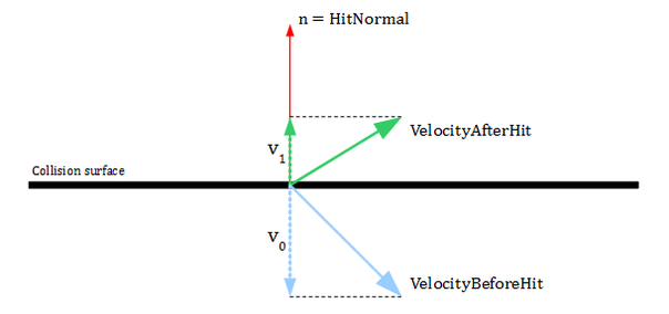
To compute the velocity after the impact, we need to assume that we want to apply an impulse along the vector n (HitNormal) with unknown magnitude j to change the velocity:

We start our computations with the main equation defining coefficient of restitution as a relation between relative velocities:

In general, relative velocities  and  are computed as projections onto the collision normal of differences between velocities for two colliding objects (symbol  is the dot product):

But in our case, because we collide only with a static environment (object B has always zero velocities), it can be simplified to:

Combining three equations together we obtain:

Now we are using the first equation and making a substitution for VelocityAfterHit:

The left side transformation:

We move the first term to the right side:

Because the collision normal n is a unit vector, it has length 1, so  is also 1:

Finally, we can simplify the right side:

Going back and making a substitution for j in the first equation:

This equation is implemented in the code as the line:

Velocity += -(1+Restitution) * ProjectedVelocity * HitInfo.normal;

This concludes the details of the collision response.

Summarizing this section, we can observe that our function calculates the full predicted trajectory for the projectile. The value of variable Position can be stored at the end of every iteration as a consecutive point of the curve. We can use it to draw the expected trajectory when a player is aiming to throw a grenade. Also, we can send the final position to the AI system to mark places to avoid.

Vehicle

When predicting the movement of the vehicle, we will consider only a short amount of prediction time. Unlike previous cases, we need to consider an angular velocity [6]. Vehicles are usually relatively big objects in the game and turning is an essential part of their movement. Hence, even if we consider a short time of prediction (less than 1 s), we still need to calculate the rotational component of the movement.

Angular velocity is the rate of change of orientation in respect to time. Angular velocity is an equivalent to linear velocity but for rotational movement. Angular velocity is a vector quantity. The direction of the vector represents the axis of rotation, and the length of the vector tells us about the rate of change of orientation – in radians per seconds.

To calculate the full predicted state of the vehicle we need to compute both components of movement: linear and rotational. Linear component (predicted position) can be evaluated in the same way as for characters. For the rotational component, we will assume the constant value of angular velocity during the prediction. The code is presented below:

Quaternion RotationalMovementPrediction(Quaternion CurrentOrientation, Vector3 AngularVelocity, float PredictionTime)
{
    float RotationAngle = AngularVelocity.magnitude * PredictionTime;
    Vector3 RotationAxis = AngularVelocity.normalized;

    Quaternion RotationFromAngularVelocity = Quaternion.AngleAxis(RotationAngle * Mathf.Rad2Deg, RotationAxis);

    Quaternion PredictedOrientation = CurrentOrientation * RotationFromAngularVelocity;
    return PredictedOrientation;
}

We build rotation quaternion using the axis and angle interface - the method Quaternion.AngleAxis(). The axis of rotation is taken directly from angular velocity as a normalized vector:

RotationAxis = AngularVelocity.normalized;

The angle of rotation is computed as the multiplication of the rate of change and our prediction time:

RotationAngle = AngularVelocity.magnitude * PredictionTime;

Since the length of angular velocity vector represents the rate of change of the orientation, if we multiply it by our desired time of prediction, the output is the total angle we need to rotate around the axis. For example, let us assume that our vehicle is turning with a rate 0.25 radians per second. If we multiply it by 2 s of prediction time, then we get 0.5 radians as the value of the RotationAngle variable (approximately 28.6 degrees). This is the predicted angle the vehicle will turn in 2 s.

Having the rotation axis and the rotation angle, we can build the quaternion from angular velocity (also, using conversion from radians to degrees, because the Unity method expects the angle in degrees as an input):

RotationFromAngularVelocity = Quaternion.AngleAxis(RotationAngle * Mathf.Rad2Deg, RotationAxis);

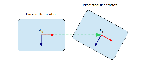
Finally, we need to compute the quaternion to represent the final predicted state. We will use multiplication, which represents a composition of two orientations. Therefore, we multiply the current orientation by the rotation quaternion, which represents the change from angular velocity:

PredictedOrientation = CurrentOrientation * RotationFromAngularVelocity;

The result of this multiplication is the orientation of the predicted state of the vehicle:

Iterations

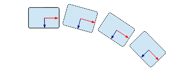
While executing rotational prediction once will give us a good approximation, for objects like cars or tanks, we might need to execute the prediction several times with smaller time steps. Also, linear velocity in vehicles is aligned with their forward direction, and it changes with every orientation change. To achieve better results - especially for a longer prediction time - we can execute both linear and rotational prediction in a loop with just a few iterations. In every iteration, we will match the linear velocity with the new forward direction from orientation to approximate the behavior of vehicle physics. The code is:

void VehicleMovementPrediction(Vector3 Position, Vector3 LinearVelocity, Quaternion Orientation, Vector3 AngularVelocity, float PredictionTime, int NumberOfIterations, out Vector3 outPosition, out Quaternion outOrientation)
{
    float DeltaTime = PredictionTime / NumberOfIterations;
    for (int i=1 ; i<=NumberOfIterations ; ++i)
    {
        Position = LinearMovementPrediction(Position, LinearVelocity, DeltaTime);
        Orientation = RotationalMovementPrediction(Orientation, AngularVelocity, DeltaTime);

        // Match LinearVelocity with the new forward direction from Orientation.
        LinearVelocity = Orientation * new Vector3(0.0f, 0.0f, LinearVelocity.magnitude);
    }

    outPosition = Position;
    outOrientation = Orientation;
}

After executing the loop, we should see prediction results similar to the image below:

Conclusion

We have presented three different scenarios for movement prediction. What they have in common is that they all perform simplified physics simulation customized for prediction needs. However, it is important to remember that this is only a prediction and it is impossible to fully predict the future of an interactive world controlled by human players. Our gameplay logic, which relies on prediction results, needs to be prepared for a failure and be ready to deliver a fail-safe solution.

Thanks

I would like to thank Luis Bermudez, Mohammed Yassir Ouali, and Philippe Baron for their valuable feedback.

References

[1] “Velocity”, https://en.wikipedia.org/wiki/Velocity

[2] “Dead reckoning”, https://en.wikipedia.org/wiki/Dead_reckoning

[3] “Latency Compensating Methods in Client/Server In-game Protocol Design and Optimization”, https://developer.valvesoftware.com/wiki/Latency_Compensating_Methods_in_Client/Server_In-game_Protocol_Design_and_Optimization

[4] “Equations of motion”, https://en.wikipedia.org/wiki/Equations_of_motion

[5] “Coefficient of restitution”, https://en.wikipedia.org/wiki/Coefficient_of_restitution

[6] “Angular velocity”, https://en.wikipedia.org/wiki/Angular_velocity